

8.4 Oscillating 1D Systems: A Second Order ODE
245
Fig. 8.21 Adjusted method: first three periods (left) and period 36–40 (right)
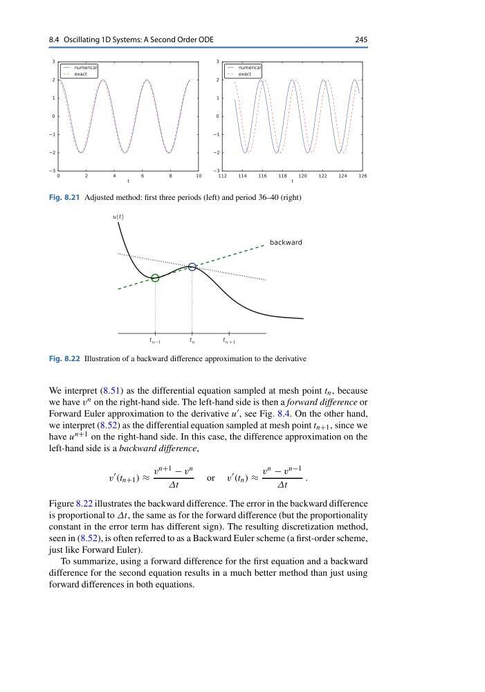
Fig. 8.22 Illustration of a backward difference approximation to the derivative
We interpret (8.51) as the differential equation sampled at mesh point t n , because
we have v n on the right-hand side. The left-hand side is then a forward difference or
Forward Euler approximation to the derivative u , see Fig. 8.4. On the other hand,
we interpret (8.52) as the differential equation sampled at mesh point t n+1 , since we
have u n+1 on the right-hand side. In this case, the difference approximation on the
left-hand side is a backward difference,
v
(t n+1 ) ≈
v n+1 − v n
Δt
or v
(t n ) ≈
v n − v n−1
Δt
.
Figure 8.22 illustrates the backward difference. The error in the backward difference
is proportional to Δt, the same as for the forward difference (but the proportionality
constant in the error term has different sign). The resulting discretization method,
seen in (8.52), is often referred to as a Backward Euler scheme (a first-order scheme,
just like Forward Euler).
To summarize, using a forward difference for the first equation and a backward
difference for the second equation results in a much better method than just using
forward differences in both equations.
245
Fig. 8.21 Adjusted method: first three periods (left) and period 36–40 (right)
Fig. 8.22 Illustration of a backward difference approximation to the derivative
We interpret (8.51) as the differential equation sampled at mesh point t n , because
we have v n on the right-hand side. The left-hand side is then a forward difference or
Forward Euler approximation to the derivative u , see Fig. 8.4. On the other hand,
we interpret (8.52) as the differential equation sampled at mesh point t n+1 , since we
have u n+1 on the right-hand side. In this case, the difference approximation on the
left-hand side is a backward difference,
v
(t n+1 ) ≈
v n+1 − v n
Δt
or v
(t n ) ≈
v n − v n−1
Δt
.
Figure 8.22 illustrates the backward difference. The error in the backward difference
is proportional to Δt, the same as for the forward difference (but the proportionality
constant in the error term has different sign). The resulting discretization method,
seen in (8.52), is often referred to as a Backward Euler scheme (a first-order scheme,
just like Forward Euler).
To summarize, using a forward difference for the first equation and a backward
difference for the second equation results in a much better method than just using
forward differences in both equations.