

244
8 Solving Ordinary Differential Equations
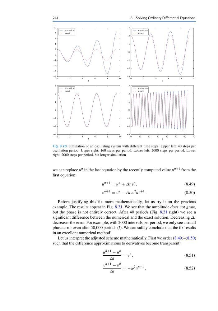
Fig. 8.20 Simulation of an oscillating system with different time steps. Upper left: 40 steps per
oscillation period. Upper right: 160 steps per period. Lower left: 2000 steps per period. Lower
right: 2000 steps per period, but longer simulation
we can replace u n in the last equation by the recently computed value u n+1 from the
first equation:
u
n+1
= u
n
+ Δt v
n ,
(8.49)
v
n+1
= v
n
− Δt ω
2 u
n+1 .
(8.50)
Before justifying this fix more mathematically, let us try it on the previous
example. The results appear in Fig. 8.21. We see that the amplitude does not grow,
but the phase is not entirely correct. After 40 periods (Fig. 8.21 right) we see a
significant difference between the numerical and the exact solution. Decreasing Δt
decreases the error. For example, with 2000 intervals per period, we only see a small
phase error even after 50,000 periods (!). We can safely conclude that the fix results
in an excellent numerical method!
Let us interpret the adjusted scheme mathematically. First we order (8.49)–(8.50)
such that the difference approximations to derivatives become transparent:
u n+1 − u n
Δt
= v
n ,
(8.51)
v n+1 − v n
Δt
= −ω
2 u
n+1 .
(8.52)
8 Solving Ordinary Differential Equations
Fig. 8.20 Simulation of an oscillating system with different time steps. Upper left: 40 steps per
oscillation period. Upper right: 160 steps per period. Lower left: 2000 steps per period. Lower
right: 2000 steps per period, but longer simulation
we can replace u n in the last equation by the recently computed value u n+1 from the
first equation:
u
n+1
= u
n
+ Δt v
n ,
(8.49)
v
n+1
= v
n
− Δt ω
2 u
n+1 .
(8.50)
Before justifying this fix more mathematically, let us try it on the previous
example. The results appear in Fig. 8.21. We see that the amplitude does not grow,
but the phase is not entirely correct. After 40 periods (Fig. 8.21 right) we see a
significant difference between the numerical and the exact solution. Decreasing Δt
decreases the error. For example, with 2000 intervals per period, we only see a small
phase error even after 50,000 periods (!). We can safely conclude that the fix results
in an excellent numerical method!
Let us interpret the adjusted scheme mathematically. First we order (8.49)–(8.50)
such that the difference approximations to derivatives become transparent:
u n+1 − u n
Δt
= v
n ,
(8.51)
v n+1 − v n
Δt
= −ω
2 u
n+1 .
(8.52)