

8.4 Oscillating 1D Systems: A Second Order ODE
243
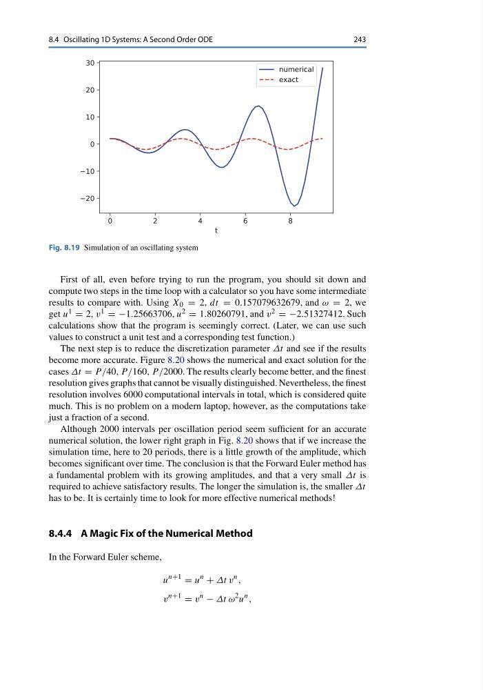
Fig. 8.19 Simulation of an oscillating system
First of all, even before trying to run the program, you should sit down and
compute two steps in the time loop with a calculator so you have some intermediate
results to compare with. Using X 0 = 2, dt = 0.157079632679, and ω = 2, we
get u 1 = 2, v 1 = −1.25663706, u 2 = 1.80260791, and v 2 = −2.51327412. Such
calculations show that the program is seemingly correct. (Later, we can use such
values to construct a unit test and a corresponding test function.)
The next step is to reduce the discretization parameter Δt and see if the results
become more accurate. Figure 8.20 shows the numerical and exact solution for the
cases Δt = P /40, P /160, P /2000. The results clearly become better, and the finest
resolution gives graphs that cannot be visually distinguished. Nevertheless, the finest
resolution involves 6000 computational intervals in total, which is considered quite
much. This is no problem on a modern laptop, however, as the computations take
just a fraction of a second.
Although 2000 intervals per oscillation period seem sufficient for an accurate
numerical solution, the lower right graph in Fig. 8.20 shows that if we increase the
simulation time, here to 20 periods, there is a little growth of the amplitude, which
becomes significant over time. The conclusion is that the Forward Euler method has
a fundamental problem with its growing amplitudes, and that a very small Δt is
required to achieve satisfactory results. The longer the simulation is, the smaller Δt
has to be. It is certainly time to look for more effective numerical methods!
8.4.4 A Magic Fix of the Numerical Method
In the Forward Euler scheme,
u
n+1
= u
n
+ Δt v
n ,
v
n+1
= v
n
− Δt ω
2 u
n ,
243
Fig. 8.19 Simulation of an oscillating system
First of all, even before trying to run the program, you should sit down and
compute two steps in the time loop with a calculator so you have some intermediate
results to compare with. Using X 0 = 2, dt = 0.157079632679, and ω = 2, we
get u 1 = 2, v 1 = −1.25663706, u 2 = 1.80260791, and v 2 = −2.51327412. Such
calculations show that the program is seemingly correct. (Later, we can use such
values to construct a unit test and a corresponding test function.)
The next step is to reduce the discretization parameter Δt and see if the results
become more accurate. Figure 8.20 shows the numerical and exact solution for the
cases Δt = P /40, P /160, P /2000. The results clearly become better, and the finest
resolution gives graphs that cannot be visually distinguished. Nevertheless, the finest
resolution involves 6000 computational intervals in total, which is considered quite
much. This is no problem on a modern laptop, however, as the computations take
just a fraction of a second.
Although 2000 intervals per oscillation period seem sufficient for an accurate
numerical solution, the lower right graph in Fig. 8.20 shows that if we increase the
simulation time, here to 20 periods, there is a little growth of the amplitude, which
becomes significant over time. The conclusion is that the Forward Euler method has
a fundamental problem with its growing amplitudes, and that a very small Δt is
required to achieve satisfactory results. The longer the simulation is, the smaller Δt
has to be. It is certainly time to look for more effective numerical methods!
8.4.4 A Magic Fix of the Numerical Method
In the Forward Euler scheme,
u
n+1
= u
n
+ Δt v
n ,
v
n+1
= v
n
− Δt ω
2 u
n ,