

242
8 Solving Ordinary Differential Equations
resulting in the computational scheme
u
n+1
= u
n
+ Δt v
n ,
(8.47)
v
n+1
= v
n
− Δt ω
2 u
n .
(8.48)
8.4.3 Programming the FE Scheme; the Special Case
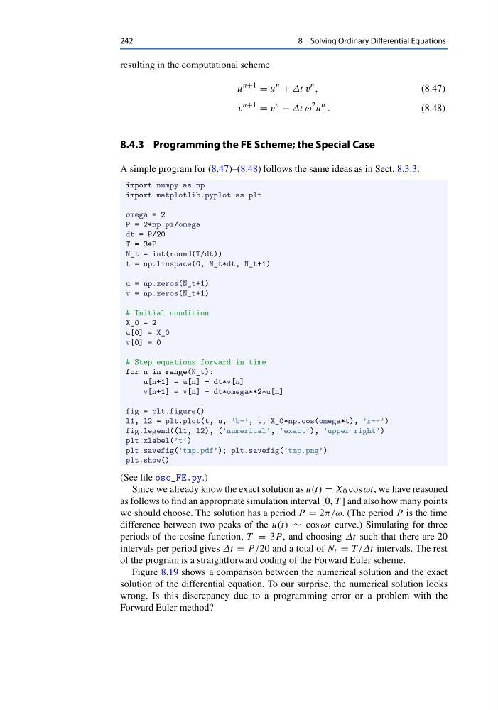
A simple program for (8.47)–(8.48) follows the same ideas as in Sect. 8.3.3:
import numpy as np
import matplotlib.pyplot as plt
omega = 2
P = 2*np.pi/omega
dt = P/20
T = 3*P
N_t = int(round(T/dt))
t = np.linspace(0, N_t*dt, N_t+1)
u = np.zeros(N_t+1)
v = np.zeros(N_t+1)
# Initial condition
X_0 = 2
u[0] = X_0
v[0] = 0
# Step equations forward in time
for n in range(N_t):
u[n+1] = u[n] + dt*v[n]
v[n+1] = v[n] - dt*omega**2*u[n]
fig = plt.figure()
l1, l2 = plt.plot(t, u, ’b-’, t, X_0*np.cos(omega*t), ’r--’)
fig.legend((l1, l2), (’numerical’, ’exact’), ’upper right’)
plt.xlabel(’t’)
plt.savefig(’tmp.pdf’); plt.savefig(’tmp.png’)
plt.show()
(See file osc_FE.py.)
Since we already know the exact solution as u(t) = X 0 cos ωt, we have reasoned
as follows to find an appropriate simulation interval [0, T ] and also how many points
we should choose. The solution has a period P = 2π/ω. (The period P is the time
difference between two peaks of the u(t) ∼ cos ωt curve.) Simulating for three
periods of the cosine function, T = 3P , and choosing Δt such that there are 20
intervals per period gives Δt = P /20 and a total of N t = T /Δt intervals. The rest
of the program is a straightforward coding of the Forward Euler scheme.
Figure 8.19 shows a comparison between the numerical solution and the exact
solution of the differential equation. To our surprise, the numerical solution looks
wrong. Is this discrepancy due to a programming error or a problem with the
Forward Euler method?
8 Solving Ordinary Differential Equations
resulting in the computational scheme
u
n+1
= u
n
+ Δt v
n ,
(8.47)
v
n+1
= v
n
− Δt ω
2 u
n .
(8.48)
8.4.3 Programming the FE Scheme; the Special Case
A simple program for (8.47)–(8.48) follows the same ideas as in Sect. 8.3.3:
import numpy as np
import matplotlib.pyplot as plt
omega = 2
P = 2*np.pi/omega
dt = P/20
T = 3*P
N_t = int(round(T/dt))
t = np.linspace(0, N_t*dt, N_t+1)
u = np.zeros(N_t+1)
v = np.zeros(N_t+1)
# Initial condition
X_0 = 2
u[0] = X_0
v[0] = 0
# Step equations forward in time
for n in range(N_t):
u[n+1] = u[n] + dt*v[n]
v[n+1] = v[n] - dt*omega**2*u[n]
fig = plt.figure()
l1, l2 = plt.plot(t, u, ’b-’, t, X_0*np.cos(omega*t), ’r--’)
fig.legend((l1, l2), (’numerical’, ’exact’), ’upper right’)
plt.xlabel(’t’)
plt.savefig(’tmp.pdf’); plt.savefig(’tmp.png’)
plt.show()
(See file osc_FE.py.)
Since we already know the exact solution as u(t) = X 0 cos ωt, we have reasoned
as follows to find an appropriate simulation interval [0, T ] and also how many points
we should choose. The solution has a period P = 2π/ω. (The period P is the time
difference between two peaks of the u(t) ∼ cos ωt curve.) Simulating for three
periods of the cosine function, T = 3P , and choosing Δt such that there are 20
intervals per period gives Δt = P /20 and a total of N t = T /Δt intervals. The rest
of the program is a straightforward coding of the Forward Euler scheme.
Figure 8.19 shows a comparison between the numerical solution and the exact
solution of the differential equation. To our surprise, the numerical solution looks
wrong. Is this discrepancy due to a programming error or a problem with the
Forward Euler method?