

8.4 Oscillating 1D Systems: A Second Order ODE
247
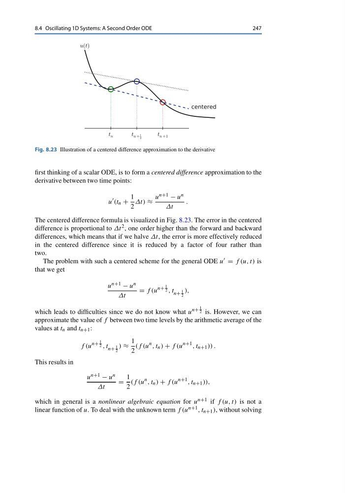
Fig. 8.23 Illustration of a centered difference approximation to the derivative
first thinking of a scalar ODE, is to form a centered difference approximation to the
derivative between two time points:
u
(t n +
1
2
Δt) ≈
u n+1 − u n
Δt
.
The centered difference formula is visualized in Fig. 8.23. The error in the centered
difference is proportional to Δt 2 , one order higher than the forward and backward
differences, which means that if we halve Δt, the error is more effectively reduced
in the centered difference since it is reduced by a factor of four rather than
two.
The problem with such a centered scheme for the general ODE u = f (u, t) is
that we get
u n+1 − u n
Δt
= f (u
n+
1
2 , t n+
1
2
),
which leads to difficulties since we do not know what u
n+
1
2 is. However, we can
approximate the value of f between two time levels by the arithmetic average of the
values at t n and t n+1 :
f (u
n+
1
2 , t n+
1
2
) ≈
1
2
(f (u
n , t n ) + f (u
n+1 , t n+1 )) .
This results in
u n+1 − u n
Δt
=
1
2
(f (u
n , t n ) + f (u
n+1 , t n+1 )),
which in general is a nonlinear algebraic equation for u n+1 if f (u, t) is not a
linear function of u. To deal with the unknown term f (u n+1 , t n+1 ), without solving
247
Fig. 8.23 Illustration of a centered difference approximation to the derivative
first thinking of a scalar ODE, is to form a centered difference approximation to the
derivative between two time points:
u
(t n +
1
2
Δt) ≈
u n+1 − u n
Δt
.
The centered difference formula is visualized in Fig. 8.23. The error in the centered
difference is proportional to Δt 2 , one order higher than the forward and backward
differences, which means that if we halve Δt, the error is more effectively reduced
in the centered difference since it is reduced by a factor of four rather than
two.
The problem with such a centered scheme for the general ODE u = f (u, t) is
that we get
u n+1 − u n
Δt
= f (u
n+
1
2 , t n+
1
2
),
which leads to difficulties since we do not know what u
n+
1
2 is. However, we can
approximate the value of f between two time levels by the arithmetic average of the
values at t n and t n+1 :
f (u
n+
1
2 , t n+
1
2
) ≈
1
2
(f (u
n , t n ) + f (u
n+1 , t n+1 )) .
This results in
u n+1 − u n
Δt
=
1
2
(f (u
n , t n ) + f (u
n+1 , t n+1 )),
which in general is a nonlinear algebraic equation for u n+1 if f (u, t) is not a
linear function of u. To deal with the unknown term f (u n+1 , t n+1 ), without solving