

320
G A R Y C . W H I T E
ine how to incorporate uncertainty of the parameter estimates into the estimates of persistence and, in the process, provide an unbiased estimate of persistence given the population model.
Any model developed to estimate population persistence has several to
many parameters that must be estimated from available data. Each of these
estimates has an associated estimate of its precision in the form of a variance,
assuming that statistically rigorous methods were used to estimate the parameter from data. In addition, because some of the parameters may have been
estimated from the same set(s) of data, some parameters in the model may
have a nonzero covariance. Thus, the vector of parameter estimates θ used in
the model to estimate persistence has the variance–covariance matrix [vâr(θ )]
to measure uncertainty.
Typically, statisticians use the delta method (Seber 1982) to estimate the
variance of a function of parameters from a set of parameter estimates and
their variance–covariance matrix. In the context of persistence, the sampling
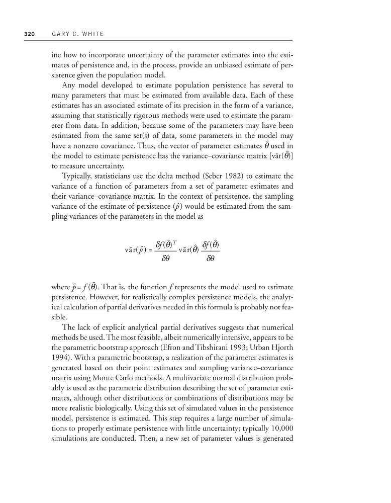
variance of the estimate of persistence (p ˆ ) would be estimated from the sampling variances of the parameters in the model as
va r(p ) = ᎏ
δf
δ
(
θ
θ ) T
ᎏ va r(θ ) ᎏ
δf
δ
(
θ
θ )
ᎏ
where p = f (θ ). That is, the function f represents the model used to estimate
persistence. However, for realistically complex persistence models, the analytical calculation of partial derivatives needed in this formula is probably not feasible.
The lack of explicit analytical partial derivatives suggests that numerical
methods be used. The most feasible, albeit numerically intensive, appears to be
the parametric bootstrap approach (Efron and Tibshirani 1993; Urban Hjorth
1994). With a parametric bootstrap, a realization of the parameter estimates is
generated based on their point estimates and sampling variance–covariance
matrix using Monte Carlo methods. A multivariate normal distribution probably is used as the parametric distribution describing the set of parameter estimates, although other distributions or combinations of distributions may be
more realistic biologically. Using this set of simulated values in the persistence
model, persistence is estimated. This step requires a large number of simulations to properly estimate persistence with little uncertainty; typically 10,000
simulations are conducted. Then, a new set of parameter values is generated
G A R Y C . W H I T E
ine how to incorporate uncertainty of the parameter estimates into the estimates of persistence and, in the process, provide an unbiased estimate of persistence given the population model.
Any model developed to estimate population persistence has several to
many parameters that must be estimated from available data. Each of these
estimates has an associated estimate of its precision in the form of a variance,
assuming that statistically rigorous methods were used to estimate the parameter from data. In addition, because some of the parameters may have been
estimated from the same set(s) of data, some parameters in the model may
have a nonzero covariance. Thus, the vector of parameter estimates θ used in
the model to estimate persistence has the variance–covariance matrix [vâr(θ )]
to measure uncertainty.
Typically, statisticians use the delta method (Seber 1982) to estimate the
variance of a function of parameters from a set of parameter estimates and
their variance–covariance matrix. In the context of persistence, the sampling
variance of the estimate of persistence (p ˆ ) would be estimated from the sampling variances of the parameters in the model as
va r(p ) = ᎏ
δf
δ
(
θ
θ ) T
ᎏ va r(θ ) ᎏ
δf
δ
(
θ
θ )
ᎏ
where p = f (θ ). That is, the function f represents the model used to estimate
persistence. However, for realistically complex persistence models, the analytical calculation of partial derivatives needed in this formula is probably not feasible.
The lack of explicit analytical partial derivatives suggests that numerical
methods be used. The most feasible, albeit numerically intensive, appears to be
the parametric bootstrap approach (Efron and Tibshirani 1993; Urban Hjorth
1994). With a parametric bootstrap, a realization of the parameter estimates is
generated based on their point estimates and sampling variance–covariance
matrix using Monte Carlo methods. A multivariate normal distribution probably is used as the parametric distribution describing the set of parameter estimates, although other distributions or combinations of distributions may be
more realistic biologically. Using this set of simulated values in the persistence
model, persistence is estimated. This step requires a large number of simulations to properly estimate persistence with little uncertainty; typically 10,000
simulations are conducted. Then, a new set of parameter values is generated