

Population Viability Analysis
321
and persistence again estimated. This process is repeated for many sets of
parameter estimates (at least 100, but more likely 1,000) to obtain a set of estimates of persistence. The variation of the resulting estimates of persistence is
then a measure of uncertainty attributable to the variation of the parameter
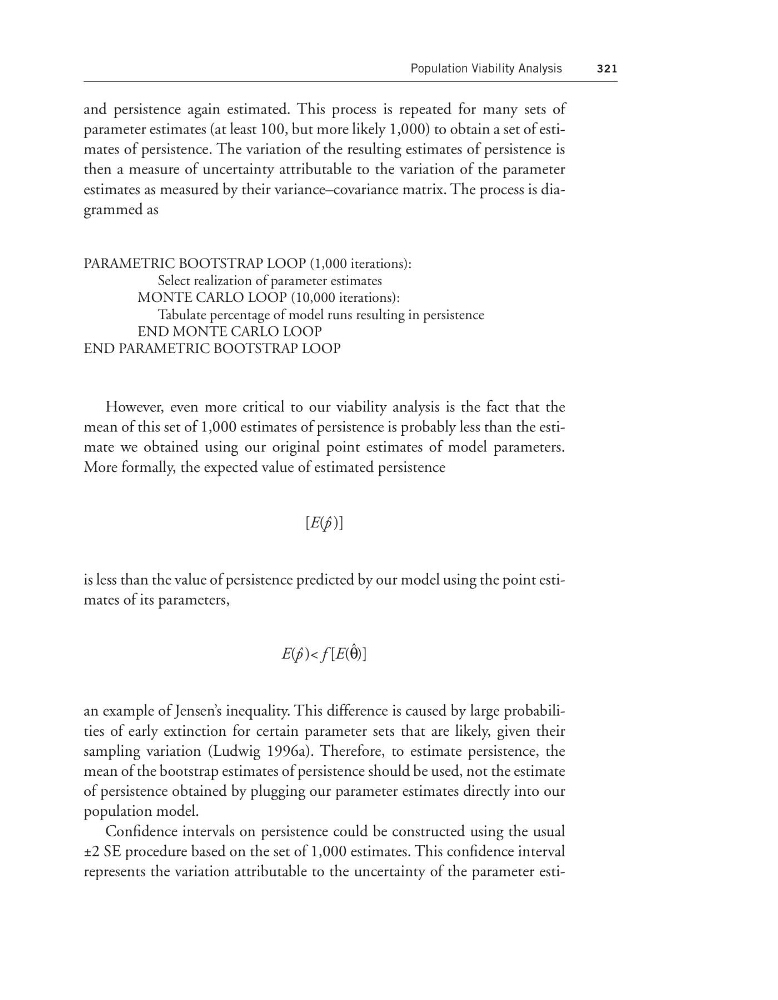
estimates as measured by their variance–covariance matrix. The process is diagrammed as
PARAMETRIC BOOTSTRAP LOOP (1,000 iterations):
Select realization of parameter estimates
MONTE CARLO LOOP (10,000 iterations):
Tabulate percentage of model runs resulting in persistence
END MONTE CARLO LOOP
END PARAMETRIC BOOTSTRAP LOOP
However, even more critical to our viability analysis is the fact that the
mean of this set of 1,000 estimates of persistence is probably less than the estimate we obtained using our original point estimates of model parameters.
More formally, the expected value of estimated persistence
[E(p ˆ )]
is less than the value of persistence predicted by our model using the point estimates of its parameters,
E(p ˆ )< f [E(θ ˆ )]
an example of Jensen’s inequality. This difference is caused by large probabilities of early extinction for certain parameter sets that are likely, given their
sampling variation (Ludwig 1996a). Therefore, to estimate persistence, the
mean of the bootstrap estimates of persistence should be used, not the estimate
of persistence obtained by plugging our parameter estimates directly into our
population model.
Confidence intervals on persistence could be constructed using the usual
±2 SE procedure based on the set of 1,000 estimates. This confidence interval
represents the variation attributable to the uncertainty of the parameter esti-
321
and persistence again estimated. This process is repeated for many sets of
parameter estimates (at least 100, but more likely 1,000) to obtain a set of estimates of persistence. The variation of the resulting estimates of persistence is
then a measure of uncertainty attributable to the variation of the parameter
estimates as measured by their variance–covariance matrix. The process is diagrammed as
PARAMETRIC BOOTSTRAP LOOP (1,000 iterations):
Select realization of parameter estimates
MONTE CARLO LOOP (10,000 iterations):
Tabulate percentage of model runs resulting in persistence
END MONTE CARLO LOOP
END PARAMETRIC BOOTSTRAP LOOP
However, even more critical to our viability analysis is the fact that the
mean of this set of 1,000 estimates of persistence is probably less than the estimate we obtained using our original point estimates of model parameters.
More formally, the expected value of estimated persistence
[E(p ˆ )]
is less than the value of persistence predicted by our model using the point estimates of its parameters,
E(p ˆ )< f [E(θ ˆ )]
an example of Jensen’s inequality. This difference is caused by large probabilities of early extinction for certain parameter sets that are likely, given their
sampling variation (Ludwig 1996a). Therefore, to estimate persistence, the
mean of the bootstrap estimates of persistence should be used, not the estimate
of persistence obtained by plugging our parameter estimates directly into our
population model.
Confidence intervals on persistence could be constructed using the usual
±2 SE procedure based on the set of 1,000 estimates. This confidence interval
represents the variation attributable to the uncertainty of the parameter esti-