

316
G A R Y C . W H I T E
R(t) = R 0΄ 1 –
ᎏ
N
K
(t)
ᎏ
θ
΅
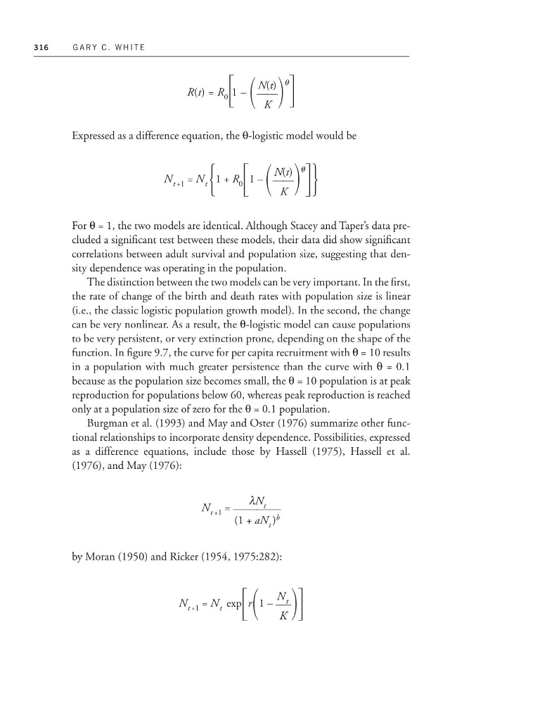
Expressed as a difference equation, the θ-logistic model would be
N t +1 = N t Ά
1 + R 0 ΄
1 –
ᎏ
N
K
(t)
ᎏ
θ
΅·
For θ = 1, the two models are identical. Although Stacey and Taper’s data precluded a significant test between these models, their data did show significant
correlations between adult survival and population size, suggesting that density dependence was operating in the population.
The distinction between the two models can be very important. In the first,
the rate of change of the birth and death rates with population size is linear
(i.e., the classic logistic population growth model). In the second, the change
can be very nonlinear. As a result, the θ-logistic model can cause populations
to be very persistent, or very extinction prone, depending on the shape of the
function. In figure 9.7, the curve for per capita recruitment with θ = 10 results
in a population with much greater persistence than the curve with θ = 0.1
because as the population size becomes small, the θ = 10 population is at peak
reproduction for populations below 60, whereas peak reproduction is reached
only at a population size of zero for the θ = 0.1 population.
Burgman et al. (1993) and May and Oster (1976) summarize other functional relationships to incorporate density dependence. Possibilities, expressed
as a difference equations, include those by Hassell (1975), Hassell et al.
(1976), and May (1976):
N t +1 = ᎏ
(1 +
λ
a
N
N
t
t ) b
ᎏ
by Moran (1950) and Ricker (1954, 1975:282):
N t +1 = N t exp
΄
r
1 – ᎏ
N
K
t
ᎏ ΅
G A R Y C . W H I T E
R(t) = R 0΄ 1 –
ᎏ
N
K
(t)
ᎏ
θ
΅
Expressed as a difference equation, the θ-logistic model would be
N t +1 = N t Ά
1 + R 0 ΄
1 –
ᎏ
N
K
(t)
ᎏ
θ
΅·
For θ = 1, the two models are identical. Although Stacey and Taper’s data precluded a significant test between these models, their data did show significant
correlations between adult survival and population size, suggesting that density dependence was operating in the population.
The distinction between the two models can be very important. In the first,
the rate of change of the birth and death rates with population size is linear
(i.e., the classic logistic population growth model). In the second, the change
can be very nonlinear. As a result, the θ-logistic model can cause populations
to be very persistent, or very extinction prone, depending on the shape of the
function. In figure 9.7, the curve for per capita recruitment with θ = 10 results
in a population with much greater persistence than the curve with θ = 0.1
because as the population size becomes small, the θ = 10 population is at peak
reproduction for populations below 60, whereas peak reproduction is reached
only at a population size of zero for the θ = 0.1 population.
Burgman et al. (1993) and May and Oster (1976) summarize other functional relationships to incorporate density dependence. Possibilities, expressed
as a difference equations, include those by Hassell (1975), Hassell et al.
(1976), and May (1976):
N t +1 = ᎏ
(1 +
λ
a
N
N
t
t ) b
ᎏ
by Moran (1950) and Ricker (1954, 1975:282):
N t +1 = N t exp
΄
r
1 – ᎏ
N
K
t
ᎏ ΅