

statement for SAS, and these included eight dummy variables to capture agroecological, cultural and socio-economic differences between communes, as well as
household size, household size squared and age of the household head. The last
control variable was a location variable showing whether a household lived in an
upland village or not, and helping to reveal differences in infrastructure access
levels between lowland and upland villages.
The panel sample was divided into two random subsamples. While two-thirds of
the panel households were used to calibrate the models, the remaining one-third
sample was used to test, out-of-sample, the predictive accuracy of the model.
In other words, sets of indicators and their parameters derived in-sample were
applied out-of-sample to predict the household poverty status. This out-of-sample
test sought to test the external validity of the tool (Johannsen 2009). For this reason,
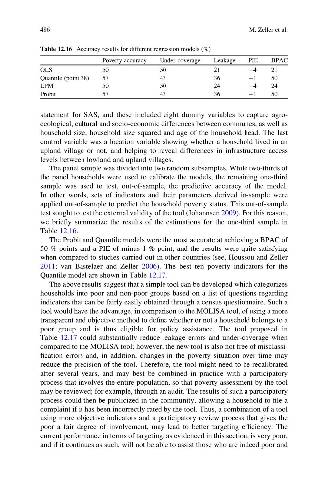
we briefly summarize the results of the estimations for the one-third sample in
Table 12.16.
The Probit and Quantile models were the most accurate at achieving a BPAC of
50 % points and a PIE of minus 1 % point, and the results were quite satisfying
when compared to studies carried out in other countries (see, Houssou and Zeller
2011; van Bastelaer and Zeller 2006). The best ten poverty indicators for the
Quantile model are shown in Table 12.17.
The above results suggest that a simple tool can be developed which categorizes
households into poor and non-poor groups based on a list of questions regarding
indicators that can be fairly easily obtained through a census questionnaire. Such a
tool would have the advantage, in comparison to the MOLISA tool, of using a more
transparent and objective method to define whether or not a household belongs to a
poor group and is thus eligible for policy assistance. The tool proposed in
Table 12.17 could substantially reduce leakage errors and under-coverage when
compared to the MOLISA tool; however, the new tool is also not free of misclassification errors and, in addition, changes in the poverty situation over time may
reduce the precision of the tool. Therefore, the tool might need to be recalibrated
after several years, and may best be combined in practice with a participatory
process that involves the entire population, so that poverty assessment by the tool
may be reviewed; for example, through an audit. The results of such a participatory
process could then be publicized in the community, allowing a household to file a
complaint if it has been incorrectly rated by the tool. Thus, a combination of a tool
using more objective indicators and a participatory review process that gives the
poor a fair degree of involvement, may lead to better targeting efficiency. The
current performance in terms of targeting, as evidenced in this section, is very poor,
and if it continues as such, will not be able to assist those who are indeed poor and
Table 12.16 Accuracy results for different regression models (%)
Poverty accuracy
Under-coverage
Leakage
PIE
BPAC
OLS
50
50
21
À4
21
Quantile (point 38)
57
43
36
À1
50
LPM
50
50
24
À4
24
Probit
57
43
36
À1
50
486
M. Zeller et al.
household size, household size squared and age of the household head. The last
control variable was a location variable showing whether a household lived in an
upland village or not, and helping to reveal differences in infrastructure access
levels between lowland and upland villages.
The panel sample was divided into two random subsamples. While two-thirds of
the panel households were used to calibrate the models, the remaining one-third
sample was used to test, out-of-sample, the predictive accuracy of the model.
In other words, sets of indicators and their parameters derived in-sample were
applied out-of-sample to predict the household poverty status. This out-of-sample
test sought to test the external validity of the tool (Johannsen 2009). For this reason,
we briefly summarize the results of the estimations for the one-third sample in
Table 12.16.
The Probit and Quantile models were the most accurate at achieving a BPAC of
50 % points and a PIE of minus 1 % point, and the results were quite satisfying
when compared to studies carried out in other countries (see, Houssou and Zeller
2011; van Bastelaer and Zeller 2006). The best ten poverty indicators for the
Quantile model are shown in Table 12.17.
The above results suggest that a simple tool can be developed which categorizes
households into poor and non-poor groups based on a list of questions regarding
indicators that can be fairly easily obtained through a census questionnaire. Such a
tool would have the advantage, in comparison to the MOLISA tool, of using a more
transparent and objective method to define whether or not a household belongs to a
poor group and is thus eligible for policy assistance. The tool proposed in
Table 12.17 could substantially reduce leakage errors and under-coverage when
compared to the MOLISA tool; however, the new tool is also not free of misclassification errors and, in addition, changes in the poverty situation over time may
reduce the precision of the tool. Therefore, the tool might need to be recalibrated
after several years, and may best be combined in practice with a participatory
process that involves the entire population, so that poverty assessment by the tool
may be reviewed; for example, through an audit. The results of such a participatory
process could then be publicized in the community, allowing a household to file a
complaint if it has been incorrectly rated by the tool. Thus, a combination of a tool
using more objective indicators and a participatory review process that gives the
poor a fair degree of involvement, may lead to better targeting efficiency. The
current performance in terms of targeting, as evidenced in this section, is very poor,
and if it continues as such, will not be able to assist those who are indeed poor and
Table 12.16 Accuracy results for different regression models (%)
Poverty accuracy
Under-coverage
Leakage
PIE
BPAC
OLS
50
50
21
À4
21
Quantile (point 38)
57
43
36
À1
50
LPM
50
50
24
À4
24
Probit
57
43
36
À1
50
486
M. Zeller et al.