

456
7 Applications: Pebble Flow Optimizations
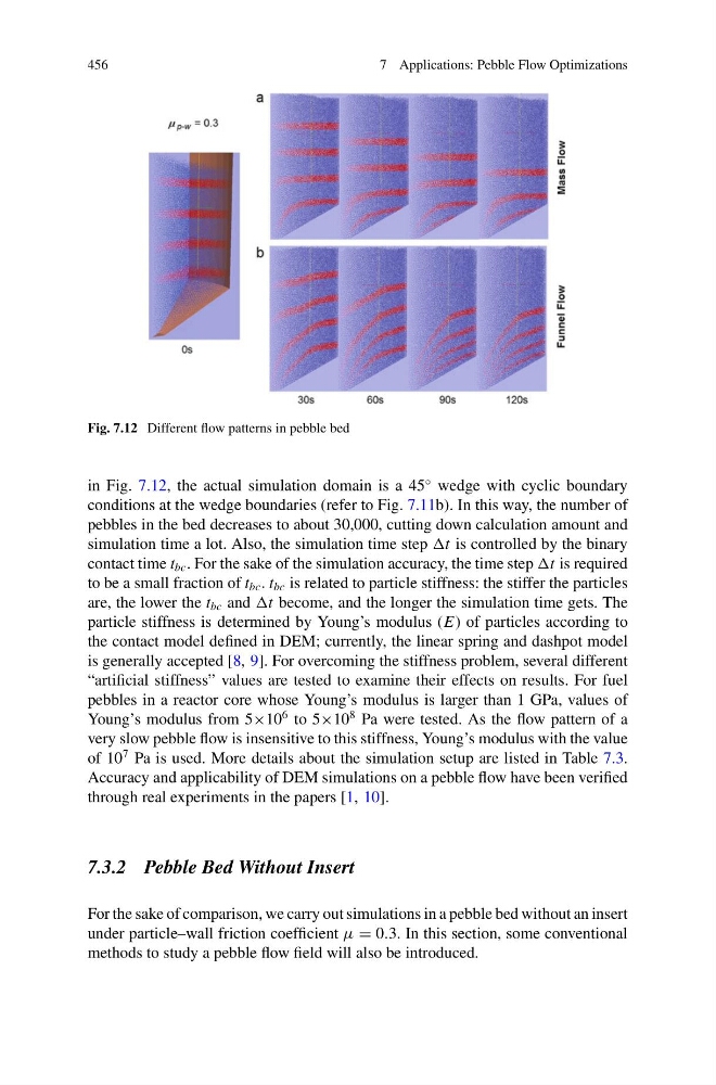
Fig. 7.12 Different flow patterns in pebble bed
in Fig. 7.12, the actual simulation domain is a 45
◦ wedge with cyclic boundary
conditions at the wedge boundaries (refer to Fig. 7.11b). In this way, the number of
pebbles in the bed decreases to about 30,000, cutting down calculation amount and
simulation time a lot. Also, the simulation time step t is controlled by the binary
contact time t bc . For the sake of the simulation accuracy, the time step t is required
to be a small fraction of t bc . t bc is related to particle stiffness: the stiffer the particles
are, the lower the t bc and t become, and the longer the simulation time gets. The
particle stiffness is determined by Young’s modulus (E) of particles according to
the contact model defined in DEM; currently, the linear spring and dashpot model
is generally accepted [8, 9]. For overcoming the stiffness problem, several different
“artificial stiffness” values are tested to examine their effects on results. For fuel
pebbles in a reactor core whose Young’s modulus is larger than 1 GPa, values of
Young’s modulus from 5×10
6 to 5×10
8 Pa were tested. As the flow pattern of a
very slow pebble flow is insensitive to this stiffness, Young’s modulus with the value
of 10
7 Pa is used. More details about the simulation setup are listed in Table 7.3.
Accuracy and applicability of DEM simulations on a pebble flow have been verified
through real experiments in the papers [1, 10].
7.3.2 Pebble Bed Without Insert
For the sake of comparison, we carry out simulations in a pebble bed without an insert
under particle–wall friction coefficient μ = 0.3. In this section, some conventional
methods to study a pebble flow field will also be introduced.
7 Applications: Pebble Flow Optimizations
Fig. 7.12 Different flow patterns in pebble bed
in Fig. 7.12, the actual simulation domain is a 45
◦ wedge with cyclic boundary
conditions at the wedge boundaries (refer to Fig. 7.11b). In this way, the number of
pebbles in the bed decreases to about 30,000, cutting down calculation amount and
simulation time a lot. Also, the simulation time step t is controlled by the binary
contact time t bc . For the sake of the simulation accuracy, the time step t is required
to be a small fraction of t bc . t bc is related to particle stiffness: the stiffer the particles
are, the lower the t bc and t become, and the longer the simulation time gets. The
particle stiffness is determined by Young’s modulus (E) of particles according to
the contact model defined in DEM; currently, the linear spring and dashpot model
is generally accepted [8, 9]. For overcoming the stiffness problem, several different
“artificial stiffness” values are tested to examine their effects on results. For fuel
pebbles in a reactor core whose Young’s modulus is larger than 1 GPa, values of
Young’s modulus from 5×10
6 to 5×10
8 Pa were tested. As the flow pattern of a
very slow pebble flow is insensitive to this stiffness, Young’s modulus with the value
of 10
7 Pa is used. More details about the simulation setup are listed in Table 7.3.
Accuracy and applicability of DEM simulations on a pebble flow have been verified
through real experiments in the papers [1, 10].
7.3.2 Pebble Bed Without Insert
For the sake of comparison, we carry out simulations in a pebble bed without an insert
under particle–wall friction coefficient μ = 0.3. In this section, some conventional
methods to study a pebble flow field will also be introduced.