

364
5 Numerical Models for Pebble-Bed Heat Transfer
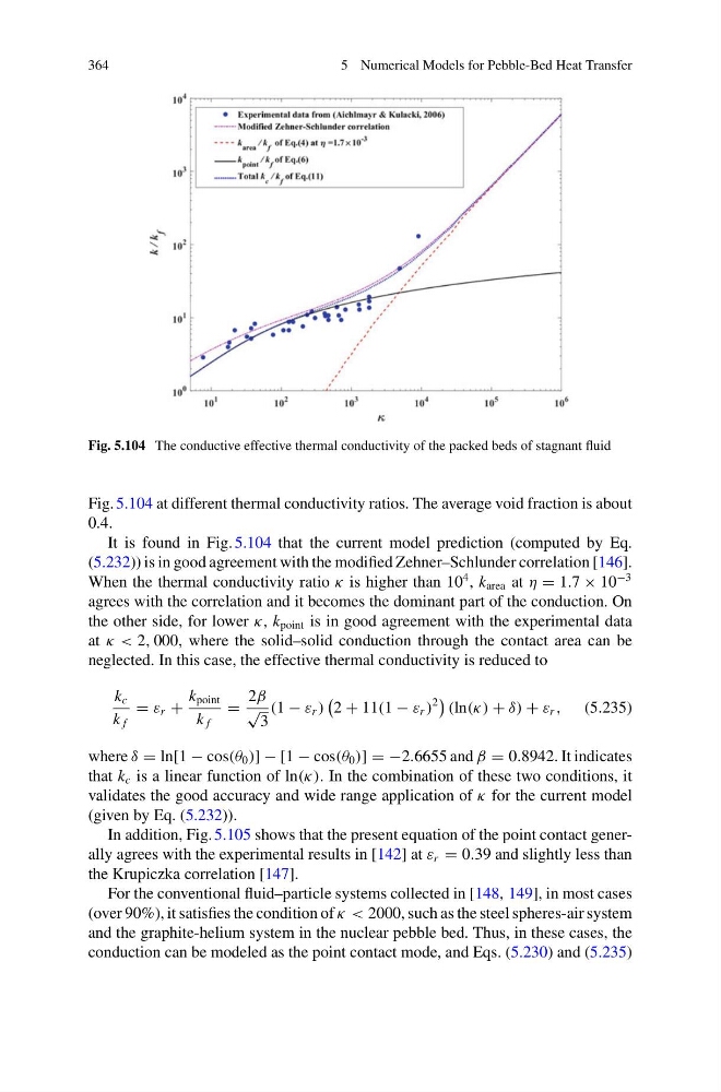
Fig. 5.104 The conductive effective thermal conductivity of the packed beds of stagnant fluid
Fig. 5.104 at different thermal conductivity ratios. The average void fraction is about
0.4.
It is found in Fig. 5.104 that the current model prediction (computed by Eq.
(5.232)) is in good agreement with the modified Zehner–Schlunder correlation [146].
When the thermal conductivity ratio κ is higher than 10
4 , k area at η = 1.7 × 10
−3
agrees with the correlation and it becomes the dominant part of the conduction. On
the other side, for lower κ, k point is in good agreement with the experimental data
at κ < 2, 000, where the solid–solid conduction through the contact area can be
neglected. In this case, the effective thermal conductivity is reduced to
k c
k f
= ε r +
k point
k f
=
2β
√
3
(1 − ε r )
2 + 11(1 − ε r )
2
(ln(κ) + δ) + ε r , (5.235)
where δ = ln[1 − cos(θ 0 )] − [1 − cos(θ 0 )] = −2.6655 and β = 0.8942. It indicates
that k c is a linear function of ln(κ). In the combination of these two conditions, it
validates the good accuracy and wide range application of κ for the current model
(given by Eq. (5.232)).
In addition, Fig. 5.105 shows that the present equation of the point contact generally agrees with the experimental results in [142] at ε r = 0.39 and slightly less than
the Krupiczka correlation [147].
For the conventional fluid–particle systems collected in [148, 149], in most cases
(over 90%), it satisfies the condition of κ < 2000, such as the steel spheres-air system
and the graphite-helium system in the nuclear pebble bed. Thus, in these cases, the
conduction can be modeled as the point contact mode, and Eqs. (5.230) and (5.235)
5 Numerical Models for Pebble-Bed Heat Transfer
Fig. 5.104 The conductive effective thermal conductivity of the packed beds of stagnant fluid
Fig. 5.104 at different thermal conductivity ratios. The average void fraction is about
0.4.
It is found in Fig. 5.104 that the current model prediction (computed by Eq.
(5.232)) is in good agreement with the modified Zehner–Schlunder correlation [146].
When the thermal conductivity ratio κ is higher than 10
4 , k area at η = 1.7 × 10
−3
agrees with the correlation and it becomes the dominant part of the conduction. On
the other side, for lower κ, k point is in good agreement with the experimental data
at κ < 2, 000, where the solid–solid conduction through the contact area can be
neglected. In this case, the effective thermal conductivity is reduced to
k c
k f
= ε r +
k point
k f
=
2β
√
3
(1 − ε r )
2 + 11(1 − ε r )
2
(ln(κ) + δ) + ε r , (5.235)
where δ = ln[1 − cos(θ 0 )] − [1 − cos(θ 0 )] = −2.6655 and β = 0.8942. It indicates
that k c is a linear function of ln(κ). In the combination of these two conditions, it
validates the good accuracy and wide range application of κ for the current model
(given by Eq. (5.232)).
In addition, Fig. 5.105 shows that the present equation of the point contact generally agrees with the experimental results in [142] at ε r = 0.39 and slightly less than
the Krupiczka correlation [147].
For the conventional fluid–particle systems collected in [148, 149], in most cases
(over 90%), it satisfies the condition of κ < 2000, such as the steel spheres-air system
and the graphite-helium system in the nuclear pebble bed. Thus, in these cases, the
conduction can be modeled as the point contact mode, and Eqs. (5.230) and (5.235)