

5.4 CFD-DEM Coupled Simulation and Development
325
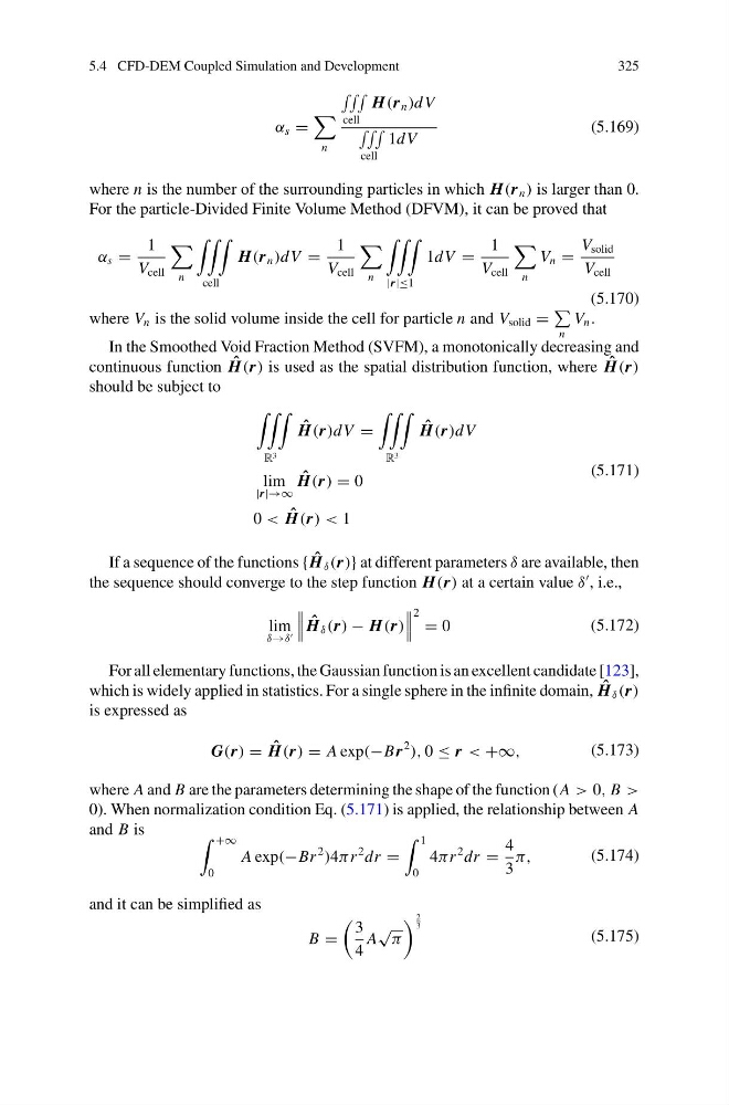
α s =
n
cell
H(r n )dV
cell
1dV
(5.169)
where n is the number of the surrounding particles in which H(r n ) is larger than 0.
For the particle-Divided Finite Volume Method (DFVM), it can be proved that
α s =
1
V cell
n
cell
H(r n )dV =
1
V cell
n
|r|≤1
1dV =
1
V cell
n
V n =
V solid
V cell
(5.170)
where V n is the solid volume inside the cell for particle n and V solid =
n
V n .
In the Smoothed Void Fraction Method (SVFM), a monotonically decreasing and
continuous function ˆ
H(r) is used as the spatial distribution function, where ˆ
H(r)
should be subject to
R 3
ˆ
H(r)dV =
R 3
ˆ
H(r)dV
lim
|r|→∞
ˆ
H(r) = 0
0 < ˆ
H(r) < 1
(5.171)
If a sequence of the functions { ˆ
H δ (r)} at different parameters δ are available, then
the sequence should converge to the step function H(r) at a certain value δ
, i.e.,
lim
δ→δ
ˆ
H δ (r) − H(r)
2 = 0
(5.172)
For all elementary functions, the Gaussian function is an excellent candidate [123],
which is widely applied in statistics. For a single sphere in the infinite domain, ˆ
H δ (r)
is expressed as
G(r) = ˆ
H(r) = A exp(−B r
2
), 0 ≤ r < +∞,
(5.173)
where A and B are the parameters determining the shape of the function ( A > 0, B >
0). When normalization condition Eq. (5.171) is applied, the relationship between A
and B is
+∞
0
A exp(−Br
2
)4πr
2 dr =
1
0
4πr
2 dr =
4
3
π,
(5.174)
and it can be simplified as
B =
3
4
A
√ π
2
3
(5.175)
325
α s =
n
cell
H(r n )dV
cell
1dV
(5.169)
where n is the number of the surrounding particles in which H(r n ) is larger than 0.
For the particle-Divided Finite Volume Method (DFVM), it can be proved that
α s =
1
V cell
n
cell
H(r n )dV =
1
V cell
n
|r|≤1
1dV =
1
V cell
n
V n =
V solid
V cell
(5.170)
where V n is the solid volume inside the cell for particle n and V solid =
n
V n .
In the Smoothed Void Fraction Method (SVFM), a monotonically decreasing and
continuous function ˆ
H(r) is used as the spatial distribution function, where ˆ
H(r)
should be subject to
R 3
ˆ
H(r)dV =
R 3
ˆ
H(r)dV
lim
|r|→∞
ˆ
H(r) = 0
0 < ˆ
H(r) < 1
(5.171)
If a sequence of the functions { ˆ
H δ (r)} at different parameters δ are available, then
the sequence should converge to the step function H(r) at a certain value δ
, i.e.,
lim
δ→δ
ˆ
H δ (r) − H(r)
2 = 0
(5.172)
For all elementary functions, the Gaussian function is an excellent candidate [123],
which is widely applied in statistics. For a single sphere in the infinite domain, ˆ
H δ (r)
is expressed as
G(r) = ˆ
H(r) = A exp(−B r
2
), 0 ≤ r < +∞,
(5.173)
where A and B are the parameters determining the shape of the function ( A > 0, B >
0). When normalization condition Eq. (5.171) is applied, the relationship between A
and B is
+∞
0
A exp(−Br
2
)4πr
2 dr =
1
0
4πr
2 dr =
4
3
π,
(5.174)
and it can be simplified as
B =
3
4
A
√ π
2
3
(5.175)