

194
4 Numerical Methods and Simulation for Pebble Flows
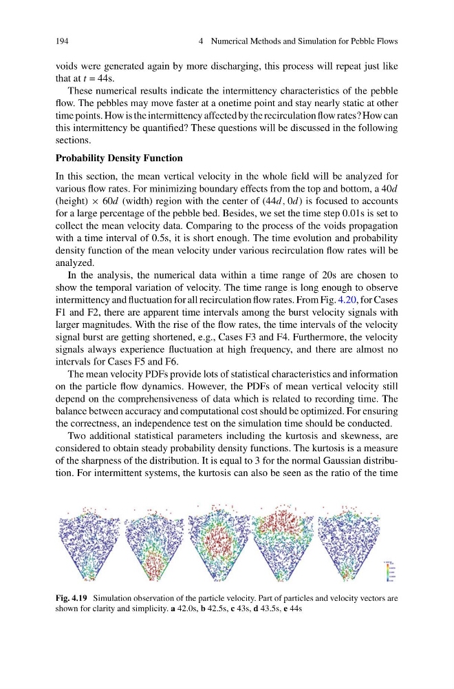
voids were generated again by more discharging, this process will repeat just like
that at t = 44s.
These numerical results indicate the intermittency characteristics of the pebble
flow. The pebbles may move faster at a onetime point and stay nearly static at other
time points. How is the intermittency affected by the recirculation flow rates? How can
this intermittency be quantified? These questions will be discussed in the following
sections.
Probability Density Function
In this section, the mean vertical velocity in the whole field will be analyzed for
various flow rates. For minimizing boundary effects from the top and bottom, a 40d
(height) × 60d (width) region with the center of (44d , 0d ) is focused to accounts
for a large percentage of the pebble bed. Besides, we set the time step 0.01s is set to
collect the mean velocity data. Comparing to the process of the voids propagation
with a time interval of 0.5s, it is short enough. The time evolution and probability
density function of the mean velocity under various recirculation flow rates will be
analyzed.
In the analysis, the numerical data within a time range of 20s are chosen to
show the temporal variation of velocity. The time range is long enough to observe
intermittency and fluctuation for all recirculation flow rates. From Fig. 4.20, for Cases
F1 and F2, there are apparent time intervals among the burst velocity signals with
larger magnitudes. With the rise of the flow rates, the time intervals of the velocity
signal burst are getting shortened, e.g., Cases F3 and F4. Furthermore, the velocity
signals always experience fluctuation at high frequency, and there are almost no
intervals for Cases F5 and F6.
The mean velocity PDFs provide lots of statistical characteristics and information
on the particle flow dynamics. However, the PDFs of mean vertical velocity still
depend on the comprehensiveness of data which is related to recording time. The
balance between accuracy and computational cost should be optimized. For ensuring
the correctness, an independence test on the simulation time should be conducted.
Two additional statistical parameters including the kurtosis and skewness, are
considered to obtain steady probability density functions. The kurtosis is a measure
of the sharpness of the distribution. It is equal to 3 for the normal Gaussian distribution. For intermittent systems, the kurtosis can also be seen as the ratio of the time
Fig. 4.19 Simulation observation of the particle velocity. Part of particles and velocity vectors are
shown for clarity and simplicity. a 42.0s, b 42.5s, c 43s, d 43.5s, e 44s
4 Numerical Methods and Simulation for Pebble Flows
voids were generated again by more discharging, this process will repeat just like
that at t = 44s.
These numerical results indicate the intermittency characteristics of the pebble
flow. The pebbles may move faster at a onetime point and stay nearly static at other
time points. How is the intermittency affected by the recirculation flow rates? How can
this intermittency be quantified? These questions will be discussed in the following
sections.
Probability Density Function
In this section, the mean vertical velocity in the whole field will be analyzed for
various flow rates. For minimizing boundary effects from the top and bottom, a 40d
(height) × 60d (width) region with the center of (44d , 0d ) is focused to accounts
for a large percentage of the pebble bed. Besides, we set the time step 0.01s is set to
collect the mean velocity data. Comparing to the process of the voids propagation
with a time interval of 0.5s, it is short enough. The time evolution and probability
density function of the mean velocity under various recirculation flow rates will be
analyzed.
In the analysis, the numerical data within a time range of 20s are chosen to
show the temporal variation of velocity. The time range is long enough to observe
intermittency and fluctuation for all recirculation flow rates. From Fig. 4.20, for Cases
F1 and F2, there are apparent time intervals among the burst velocity signals with
larger magnitudes. With the rise of the flow rates, the time intervals of the velocity
signal burst are getting shortened, e.g., Cases F3 and F4. Furthermore, the velocity
signals always experience fluctuation at high frequency, and there are almost no
intervals for Cases F5 and F6.
The mean velocity PDFs provide lots of statistical characteristics and information
on the particle flow dynamics. However, the PDFs of mean vertical velocity still
depend on the comprehensiveness of data which is related to recording time. The
balance between accuracy and computational cost should be optimized. For ensuring
the correctness, an independence test on the simulation time should be conducted.
Two additional statistical parameters including the kurtosis and skewness, are
considered to obtain steady probability density functions. The kurtosis is a measure
of the sharpness of the distribution. It is equal to 3 for the normal Gaussian distribution. For intermittent systems, the kurtosis can also be seen as the ratio of the time
Fig. 4.19 Simulation observation of the particle velocity. Part of particles and velocity vectors are
shown for clarity and simplicity. a 42.0s, b 42.5s, c 43s, d 43.5s, e 44s