

3.2 Experimental Facility and Methodology
129
If the iteration stops with the stopping criteria, the ultimate P
k , namely the effective thermal diffusivity α, is the optimal value of the inverse method.
3.2.2.3 Inverse Problem
Because the final experiment hasn’t been conducted formally at the present time,
the inverse method uses sets of temperature data from the 3D numerical simulation
experiment with an integrated model shown in Fig. (3.2). The measured points of T1–
T6 are picked to validate the availability, robustness, and accuracy of this algorithm
theoretically, and it’s also used to modify the practical experimental program. In the
simulation experiment, the constant ¯
ρ = 2250 kg/m
3 , as well as c g = 709 J/kg ·
◦ C.
Moreover, the exact parameters p e = ( p e1 , p e2 , p e3 )
T used in the simulation in Eq.
(3.7), are
p e1 = 1.7115 × 10
−6 m
2
/s,
(3.19)
p e2 = −7.5176 × 10
−10 m
2
/s ·
◦ C,
(3.20)
p e3 = 1.1671 × 10
−11 m
2
/s ·
◦ C
2
.
(3.21)
Also, since the constant density and specific heat capacity are used in this simulation,
the results and discussions of effective thermal conductivity are similar to diffusivity’s
results and discussion, and these issues of conductivity are not rephrased in this
section.
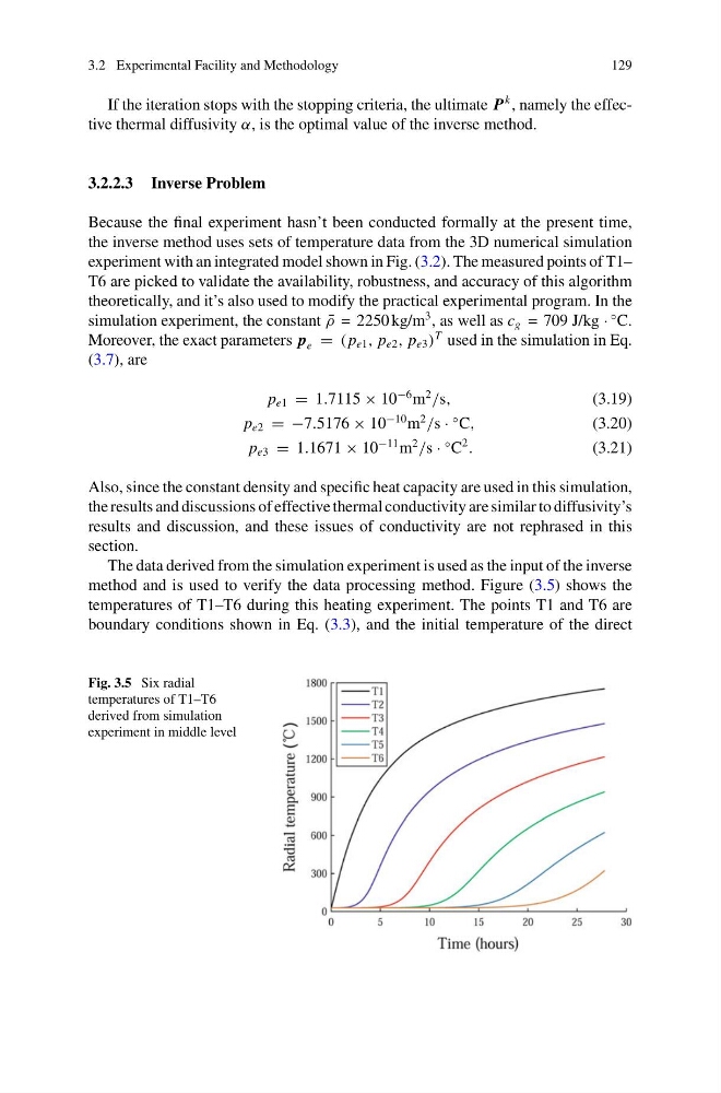
The data derived from the simulation experiment is used as the input of the inverse
method and is used to verify the data processing method. Figure (3.5) shows the
temperatures of T1–T6 during this heating experiment. The points T1 and T6 are
boundary conditions shown in Eq. (3.3), and the initial temperature of the direct
Fig. 3.5 Six radial
temperatures of T1–T6
derived from simulation
experiment in middle level
129
If the iteration stops with the stopping criteria, the ultimate P
k , namely the effective thermal diffusivity α, is the optimal value of the inverse method.
3.2.2.3 Inverse Problem
Because the final experiment hasn’t been conducted formally at the present time,
the inverse method uses sets of temperature data from the 3D numerical simulation
experiment with an integrated model shown in Fig. (3.2). The measured points of T1–
T6 are picked to validate the availability, robustness, and accuracy of this algorithm
theoretically, and it’s also used to modify the practical experimental program. In the
simulation experiment, the constant ¯
ρ = 2250 kg/m
3 , as well as c g = 709 J/kg ·
◦ C.
Moreover, the exact parameters p e = ( p e1 , p e2 , p e3 )
T used in the simulation in Eq.
(3.7), are
p e1 = 1.7115 × 10
−6 m
2
/s,
(3.19)
p e2 = −7.5176 × 10
−10 m
2
/s ·
◦ C,
(3.20)
p e3 = 1.1671 × 10
−11 m
2
/s ·
◦ C
2
.
(3.21)
Also, since the constant density and specific heat capacity are used in this simulation,
the results and discussions of effective thermal conductivity are similar to diffusivity’s
results and discussion, and these issues of conductivity are not rephrased in this
section.
The data derived from the simulation experiment is used as the input of the inverse
method and is used to verify the data processing method. Figure (3.5) shows the
temperatures of T1–T6 during this heating experiment. The points T1 and T6 are
boundary conditions shown in Eq. (3.3), and the initial temperature of the direct
Fig. 3.5 Six radial
temperatures of T1–T6
derived from simulation
experiment in middle level