

128
3 Experiments in Pebble Bed Heat Transfer
where k is the number of iterations, and μ is a positive scalar named damping
parameter.
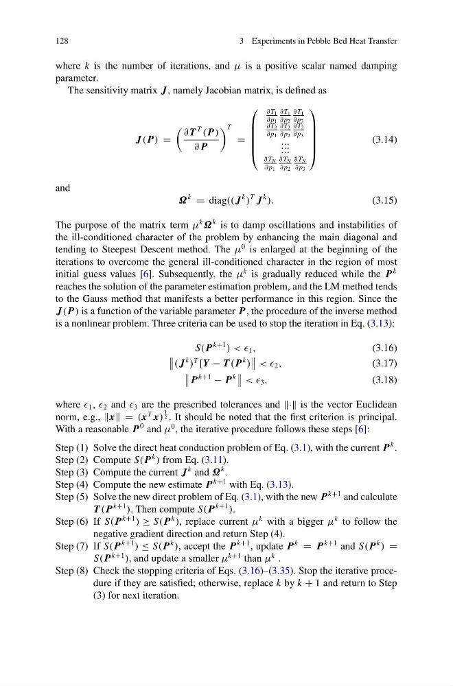
The sensitivity matrix J, namely Jacobian matrix, is defined as
J( P) =
∂ T
T
( P)
∂ P
T
=
⎛
⎜
⎜
⎜
⎜
⎝
∂ T 1
∂ p 1
∂ T 1
∂ p 2
∂ T 1
∂ p 3
∂ T 2
∂ p 1
∂ T 2
∂ p 2
∂ T 2
∂ p 3
. . .
. . .
. . .
∂ T N
∂ p 1
∂ T N
∂ p 2
∂ T N
∂ p 3
⎞
⎟
⎟
⎟
⎟
⎠
(3.14)
and
Ω
k
= diag(( J
k
)
T J
k
).
(3.15)
The purpose of the matrix term μ
k
Ω
k is to damp oscillations and instabilities of
the ill-conditioned character of the problem by enhancing the main diagonal and
tending to Steepest Descent method. The μ
0 is enlarged at the beginning of the
iterations to overcome the general ill-conditioned character in the region of most
initial guess values [6]. Subsequently, the μ
k is gradually reduced while the P
k
reaches the solution of the parameter estimation problem, and the LM method tends
to the Gauss method that manifests a better performance in this region. Since the
J( P) is a function of the variable parameter P, the procedure of the inverse method
is a nonlinear problem. Three criteria can be used to stop the iteration in Eq. (3.13):
S( P
k+1
) < < 1 ,
(3.16)
( J
k
)
T
[Y − T ( P
k
)
< < 2 ,
(3.17)
P
k+1
− P
k
< < 3 ,
(3.18)
where 1 , 2 and 3 are the prescribed tolerances and · is the vector Euclidean
norm, e.g., x = (x
T x)
1
2 . It should be noted that the first criterion is principal.
With a reasonable P
0 and μ
0 , the iterative procedure follows these steps [6]:
Step (1) Solve the direct heat conduction problem of Eq. (3.1), with the current P
k .
Step (2) Compute S( P
k
) from Eq. (3.11).
Step (3) Compute the current J
k and Ω
k .
Step (4) Compute the new estimate P
k+1 with Eq. (3.13).
Step (5) Solve the new direct problem of Eq. (3.1), with the new P
k+1 and calculate
T ( P
k+1
). Then compute S( P
k+1
).
Step (6) If S( P
k+1
) ≥ S( P
k
), replace current μ
k with a bigger μ
k to follow the
negative gradient direction and return Step (4).
Step (7) If S( P
k+1
) ≤ S( P
k
), accept the P
k+1 , update P
k
= P
k+1 and S( P
k
) =
S( P
k+1
), and update a smaller μ
k+1 than μ
k .
Step (8) Check the stopping criteria of Eqs. (3.16)–(3.35). Stop the iterative procedure if they are satisfied; otherwise, replace k by k + 1 and return to Step
(3) for next iteration.
3 Experiments in Pebble Bed Heat Transfer
where k is the number of iterations, and μ is a positive scalar named damping
parameter.
The sensitivity matrix J, namely Jacobian matrix, is defined as
J( P) =
∂ T
T
( P)
∂ P
T
=
⎛
⎜
⎜
⎜
⎜
⎝
∂ T 1
∂ p 1
∂ T 1
∂ p 2
∂ T 1
∂ p 3
∂ T 2
∂ p 1
∂ T 2
∂ p 2
∂ T 2
∂ p 3
. . .
. . .
. . .
∂ T N
∂ p 1
∂ T N
∂ p 2
∂ T N
∂ p 3
⎞
⎟
⎟
⎟
⎟
⎠
(3.14)
and
Ω
k
= diag(( J
k
)
T J
k
).
(3.15)
The purpose of the matrix term μ
k
Ω
k is to damp oscillations and instabilities of
the ill-conditioned character of the problem by enhancing the main diagonal and
tending to Steepest Descent method. The μ
0 is enlarged at the beginning of the
iterations to overcome the general ill-conditioned character in the region of most
initial guess values [6]. Subsequently, the μ
k is gradually reduced while the P
k
reaches the solution of the parameter estimation problem, and the LM method tends
to the Gauss method that manifests a better performance in this region. Since the
J( P) is a function of the variable parameter P, the procedure of the inverse method
is a nonlinear problem. Three criteria can be used to stop the iteration in Eq. (3.13):
S( P
k+1
) < < 1 ,
(3.16)
( J
k
)
T
[Y − T ( P
k
)
< < 2 ,
(3.17)
P
k+1
− P
k
< < 3 ,
(3.18)
where 1 , 2 and 3 are the prescribed tolerances and · is the vector Euclidean
norm, e.g., x = (x
T x)
1
2 . It should be noted that the first criterion is principal.
With a reasonable P
0 and μ
0 , the iterative procedure follows these steps [6]:
Step (1) Solve the direct heat conduction problem of Eq. (3.1), with the current P
k .
Step (2) Compute S( P
k
) from Eq. (3.11).
Step (3) Compute the current J
k and Ω
k .
Step (4) Compute the new estimate P
k+1 with Eq. (3.13).
Step (5) Solve the new direct problem of Eq. (3.1), with the new P
k+1 and calculate
T ( P
k+1
). Then compute S( P
k+1
).
Step (6) If S( P
k+1
) ≥ S( P
k
), replace current μ
k with a bigger μ
k to follow the
negative gradient direction and return Step (4).
Step (7) If S( P
k+1
) ≤ S( P
k
), accept the P
k+1 , update P
k
= P
k+1 and S( P
k
) =
S( P
k+1
), and update a smaller μ
k+1 than μ
k .
Step (8) Check the stopping criteria of Eqs. (3.16)–(3.35). Stop the iterative procedure if they are satisfied; otherwise, replace k by k + 1 and return to Step
(3) for next iteration.