

56
3 Microscopic Expressions of Nonlinear Polarization
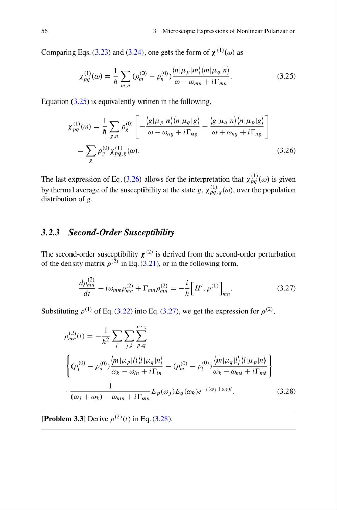
Comparing Eqs. (3.23) and (3.24), one gets the form of χ (1) (ω) as
χ
(1)
pq (ω) =
1
¯
h
m,n
(ρ
(0)
m − ρ
(0)
n )
n|μ p |m
m|μ q |n
ω − ω mn + ii mn
.
(3.25)
Equation (3.25) is equivalently written in the following,
χ
(1)
pq (ω) =
1
¯
h
g,n
ρ
(0)
g
−
g|μ p |n
n|μ q |g
ω − ω ng + ii ng
+
g|μ q |n
n|μ p |g
ω + ω ng + ii ng
=
g
ρ
(0)
g χ
(1)
pq,g (ω).
(3.26)
The last expression of Eq. (3.26) allows for the interpretation that χ
(1)
pq (ω) is given
by thermal average of the susceptibility at the state g, χ
(1)
pq,g (ω), over the population
distribution of g.
3.2.3 Second-Order Susceptibility
The second-order susceptibility χ (2) is derived from the second-order perturbation
of the density matrix ρ (2) in Eq. (3.21), or in the following form,
dρ
(2)
mn
dt
+ iω mn ρ
(2)
mn + mn ρ
(2)
mn = −
i
¯
h
H
, ρ
(1)
mn
.
(3.27)
Substituting ρ (1) of Eq. (3.22) into Eq. (3.27), we get the expression for ρ (2) ,
ρ
(2)
mn (t) = −
1
¯
h 2
l
j,k
x∼z
p,q
(ρ
(0)
l − ρ
(0)
n )
m|μ p |l
l|μ q |n
ω k − ω ln + ii ln
− (ρ
(0)
m − ρ
(0)
l )
m|μ q |l
l|μ p |n
ω k − ω ml + ii ml
·
1
(ω j + ω k ) − ω mn + ii mn
E p (ω j )E q (ω k )e
−i(ω j +ω k )t .
(3.28)
[Problem 3.3] Derive ρ (2) (t) in Eq. (3.28).
3 Microscopic Expressions of Nonlinear Polarization
Comparing Eqs. (3.23) and (3.24), one gets the form of χ (1) (ω) as
χ
(1)
pq (ω) =
1
¯
h
m,n
(ρ
(0)
m − ρ
(0)
n )
n|μ p |m
m|μ q |n
ω − ω mn + ii mn
.
(3.25)
Equation (3.25) is equivalently written in the following,
χ
(1)
pq (ω) =
1
¯
h
g,n
ρ
(0)
g
−
g|μ p |n
n|μ q |g
ω − ω ng + ii ng
+
g|μ q |n
n|μ p |g
ω + ω ng + ii ng
=
g
ρ
(0)
g χ
(1)
pq,g (ω).
(3.26)
The last expression of Eq. (3.26) allows for the interpretation that χ
(1)
pq (ω) is given
by thermal average of the susceptibility at the state g, χ
(1)
pq,g (ω), over the population
distribution of g.
3.2.3 Second-Order Susceptibility
The second-order susceptibility χ (2) is derived from the second-order perturbation
of the density matrix ρ (2) in Eq. (3.21), or in the following form,
dρ
(2)
mn
dt
+ iω mn ρ
(2)
mn + mn ρ
(2)
mn = −
i
¯
h
H
, ρ
(1)
mn
.
(3.27)
Substituting ρ (1) of Eq. (3.22) into Eq. (3.27), we get the expression for ρ (2) ,
ρ
(2)
mn (t) = −
1
¯
h 2
l
j,k
x∼z
p,q
(ρ
(0)
l − ρ
(0)
n )
m|μ p |l
l|μ q |n
ω k − ω ln + ii ln
− (ρ
(0)
m − ρ
(0)
l )
m|μ q |l
l|μ p |n
ω k − ω ml + ii ml
·
1
(ω j + ω k ) − ω mn + ii mn
E p (ω j )E q (ω k )e
−i(ω j +ω k )t .
(3.28)
[Problem 3.3] Derive ρ (2) (t) in Eq. (3.28).