

52
3 Microscopic Expressions of Nonlinear Polarization
and thereby Eq. (3.13) becomes equivalent to Eq. (3.5) in terms of the expression
of the expectation value. We note that ρ mn (t) in Eq. (3.14) does not include the
explicit bath coordinates R any more, as they are averaged out in the right hand
side. Equations (3.13) and (3.14) provide a closed description of the partial system
within the coordinates r. The density matrix for the partial system in Eq. (3.14) is
sufficient to describe the physical quantity A for the partial system, with obviating
details of the bath wavefunctions C n .
A remaining issue is to determine the time development of the density matrix thus
defined. The time development of the partial system could not be represented by the
Liouville equation (3.8) with the Hamiltonian for the partial system H , because the
time development is influenced by the interaction with the bath. One could describe
the time development using the Hamiltonian and density matrix (or wavefunction)
for the whole system, though such a way is not compatible with the merit of using
the density matrix formalism. Here we avoid the tedious route to treat the whole
system, but rather focus on the time development of the partial system itself in a
closed, phenomenological way.
When the partial system interacts with the bath, an outstanding feature arises that
the partial system approaches thermal equilibrium. This is a quite general tendency,
irrespective of the details of the interaction with the bath. The thermal equilibrium
is represented as a mixed state, where the probability of state n is proportional to
the Boltzmann factor exp(−E n /k B T ) and the off-diagonal correlation vanishes by
random fluctuation. Therefore, the thermal equilibrium is specified by the following
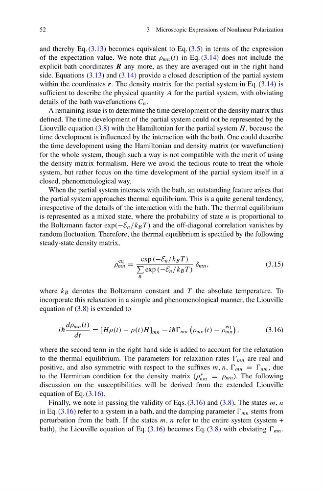
steady-state density matrix,
ρ
eq
mn =
exp (−E n /k B T )
n
exp (−E n /k B T )
δ mn ,
(3.15)
where k B denotes the Boltzmann constant and T the absolute temperature. To
incorporate this relaxation in a simple and phenomenological manner, the Liouville
equation of (3.8) is extended to
i ¯
h
dρ mn (t)
dt
= [Hρ(t) − ρ(t)H ] mn − i ¯
hh mn
ρ mn (t) − ρ
eq
mn
,
(3.16)
where the second term in the right hand side is added to account for the relaxation
to the thermal equilibrium. The parameters for relaxation rates mn are real and
positive, and also symmetric with respect to the suffixes m, n, mn = nm , due
to the Hermitian condition for the density matrix (ρ ∗
nm = ρ mn ). The following
discussion on the susceptibilities will be derived from the extended Liouville
equation of Eq. (3.16).
Finally, we note in passing the validity of Eqs. (3.16) and (3.8). The states m, n
in Eq. (3.16) refer to a system in a bath, and the damping parameter mn stems from
perturbation from the bath. If the states m, n refer to the entire system (system +
bath), the Liouville equation of Eq. (3.16) becomes Eq. (3.8) with obviating mn .
3 Microscopic Expressions of Nonlinear Polarization
and thereby Eq. (3.13) becomes equivalent to Eq. (3.5) in terms of the expression
of the expectation value. We note that ρ mn (t) in Eq. (3.14) does not include the
explicit bath coordinates R any more, as they are averaged out in the right hand
side. Equations (3.13) and (3.14) provide a closed description of the partial system
within the coordinates r. The density matrix for the partial system in Eq. (3.14) is
sufficient to describe the physical quantity A for the partial system, with obviating
details of the bath wavefunctions C n .
A remaining issue is to determine the time development of the density matrix thus
defined. The time development of the partial system could not be represented by the
Liouville equation (3.8) with the Hamiltonian for the partial system H , because the
time development is influenced by the interaction with the bath. One could describe
the time development using the Hamiltonian and density matrix (or wavefunction)
for the whole system, though such a way is not compatible with the merit of using
the density matrix formalism. Here we avoid the tedious route to treat the whole
system, but rather focus on the time development of the partial system itself in a
closed, phenomenological way.
When the partial system interacts with the bath, an outstanding feature arises that
the partial system approaches thermal equilibrium. This is a quite general tendency,
irrespective of the details of the interaction with the bath. The thermal equilibrium
is represented as a mixed state, where the probability of state n is proportional to
the Boltzmann factor exp(−E n /k B T ) and the off-diagonal correlation vanishes by
random fluctuation. Therefore, the thermal equilibrium is specified by the following
steady-state density matrix,
ρ
eq
mn =
exp (−E n /k B T )
n
exp (−E n /k B T )
δ mn ,
(3.15)
where k B denotes the Boltzmann constant and T the absolute temperature. To
incorporate this relaxation in a simple and phenomenological manner, the Liouville
equation of (3.8) is extended to
i ¯
h
dρ mn (t)
dt
= [Hρ(t) − ρ(t)H ] mn − i ¯
hh mn
ρ mn (t) − ρ
eq
mn
,
(3.16)
where the second term in the right hand side is added to account for the relaxation
to the thermal equilibrium. The parameters for relaxation rates mn are real and
positive, and also symmetric with respect to the suffixes m, n, mn = nm , due
to the Hermitian condition for the density matrix (ρ ∗
nm = ρ mn ). The following
discussion on the susceptibilities will be derived from the extended Liouville
equation of Eq. (3.16).
Finally, we note in passing the validity of Eqs. (3.16) and (3.8). The states m, n
in Eq. (3.16) refer to a system in a bath, and the damping parameter mn stems from
perturbation from the bath. If the states m, n refer to the entire system (system +
bath), the Liouville equation of Eq. (3.16) becomes Eq. (3.8) with obviating mn .