

3.1 Density Matrix
51
ψ|A|ψ =
ensemble
j,k
n,m
P
j P
k c
j
n (t)
∗ c
k
m (t)n|A|m
= A =
ensemble
j
n,m
P
j c
j
n (t)
∗ c
j
m (t)n|A|m.
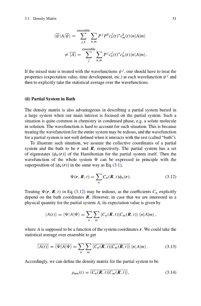
If the mixed state is treated with the wavefunctions ψ j , one should have to treat the
properties (expectation value, time development, etc.) at each wavefunction ψ j and
then to explicitly take the statistical average over the wavefunctions.
(ii) Partial System in Bath
The density matrix is also advantageous in describing a partial system buried in
a large system when our main interest is focused on the partial system. Such a
situation is quite common in chemistry in condensed phase, e.g. a solute molecule
in solution. The wavefunction is hard to account for such situation. This is because
treating the wavefunction for the entire system may be tedious, and the wavefunction
for a partial system is not well defined when it interacts with the rest (called “bath”).
To illustrate such situation, we assume the collective coordinates of a partial
system and the bath to be r and R, respectively. The partial system has a set
of eigenstates {φ n (r)} of the Hamiltonian for the partial system itself. Then the
wavefunction of the whole system can be expressed in principle with the
superposition of {φ n (r)} in the same way as Eq. (3.1),
(r, R, t) =
n
C n (R, t)φ n (r).
(3.12)
Treating (r, R, t) in Eq. (3.12) may be tedious, as the coefficients C n explicitly
depend on the bath coordinates R. However, in case that we are interested in a
physical quantity for the partial system A, its expectation value is given by
A(t) = |A| =
n
m
C n (R, t)|C m (R, t) n|A|m ,
where A is supposed to be a function of the system coordinates r. We could take the
statistical average over ensemble to get
A(t) = |A| =
n
m
C n (R, t)|C m (R, t) n|A|m .
(3.13)
Accordingly, we can define the density matrix for the partial system to be
ρ mn (t) = C n (R, t)|C m (R, t),
(3.14)
51
ψ|A|ψ =
ensemble
j,k
n,m
P
j P
k c
j
n (t)
∗ c
k
m (t)n|A|m
= A =
ensemble
j
n,m
P
j c
j
n (t)
∗ c
j
m (t)n|A|m.
If the mixed state is treated with the wavefunctions ψ j , one should have to treat the
properties (expectation value, time development, etc.) at each wavefunction ψ j and
then to explicitly take the statistical average over the wavefunctions.
(ii) Partial System in Bath
The density matrix is also advantageous in describing a partial system buried in
a large system when our main interest is focused on the partial system. Such a
situation is quite common in chemistry in condensed phase, e.g. a solute molecule
in solution. The wavefunction is hard to account for such situation. This is because
treating the wavefunction for the entire system may be tedious, and the wavefunction
for a partial system is not well defined when it interacts with the rest (called “bath”).
To illustrate such situation, we assume the collective coordinates of a partial
system and the bath to be r and R, respectively. The partial system has a set
of eigenstates {φ n (r)} of the Hamiltonian for the partial system itself. Then the
wavefunction of the whole system can be expressed in principle with the
superposition of {φ n (r)} in the same way as Eq. (3.1),
(r, R, t) =
n
C n (R, t)φ n (r).
(3.12)
Treating (r, R, t) in Eq. (3.12) may be tedious, as the coefficients C n explicitly
depend on the bath coordinates R. However, in case that we are interested in a
physical quantity for the partial system A, its expectation value is given by
A(t) = |A| =
n
m
C n (R, t)|C m (R, t) n|A|m ,
where A is supposed to be a function of the system coordinates r. We could take the
statistical average over ensemble to get
A(t) = |A| =
n
m
C n (R, t)|C m (R, t) n|A|m .
(3.13)
Accordingly, we can define the density matrix for the partial system to be
ρ mn (t) = C n (R, t)|C m (R, t),
(3.14)