

204
8 Other Topics
origin of the perturbation can be twofold, orientational and electronic mechanisms.
The former, orientational mechanism of χ (3) means that the static electric field
perturbs the orientational structure of molecules and thereby changes the χ (2) of
that material. The latter, electronic mechanism means that the electronic state of
the material has the intrinsic third-order response to the electric fields. Relative
significance of the two mechanisms in χ (3) may depend on the system in question. In
liquid water or dilute aqueous solutions, the orientational mechanism is confirmed
to be dominant in χ (3) by direct computation of the two mechanisms [16].
Third issue is the distinction of the χ (3) effect from the quadrupole terms
discussed in Chap. 7. Both the χ (3) in the present chapter and the quadrupole
terms are fourth-rank tensors and thus allowed in isotropic bulk media, though their
mechanisms are fully distinct. The χ (3) effect arises only when the electrostatic
field is imposed on the system, while the quadrupole contributions are present in the
SFG/SHG even in a system under no electrostatic field. If we take account of the
quadrupole contributions in Eqs. (8.2) and (8.3), the χ (2) in these equations should
be replaced with the extended susceptibility χ
(2)
qG in Eq. (7.50) that includes both the
dipole and quadrupole contributions.
The χ (3) formula of Eq. (8.3) allows for straightforward calculation of the χ (3)
tensor by adopting the computational methods of χ (2) in Chap. 4. One can calculate
χ (2) of a system with imposing a finite electrostatic field E(0), and take the
derivative of the calculated χ (2) with respect to the applied electrostatic field. Such
MD calculation of χ (3) is conducted using isotropic bulk systems which are free
from interfaces [16]. The calculated derivative of χ (2) derives the pure χ (3) term as
a bulk property, since the isotropic systems are essentially free from the intrinsic
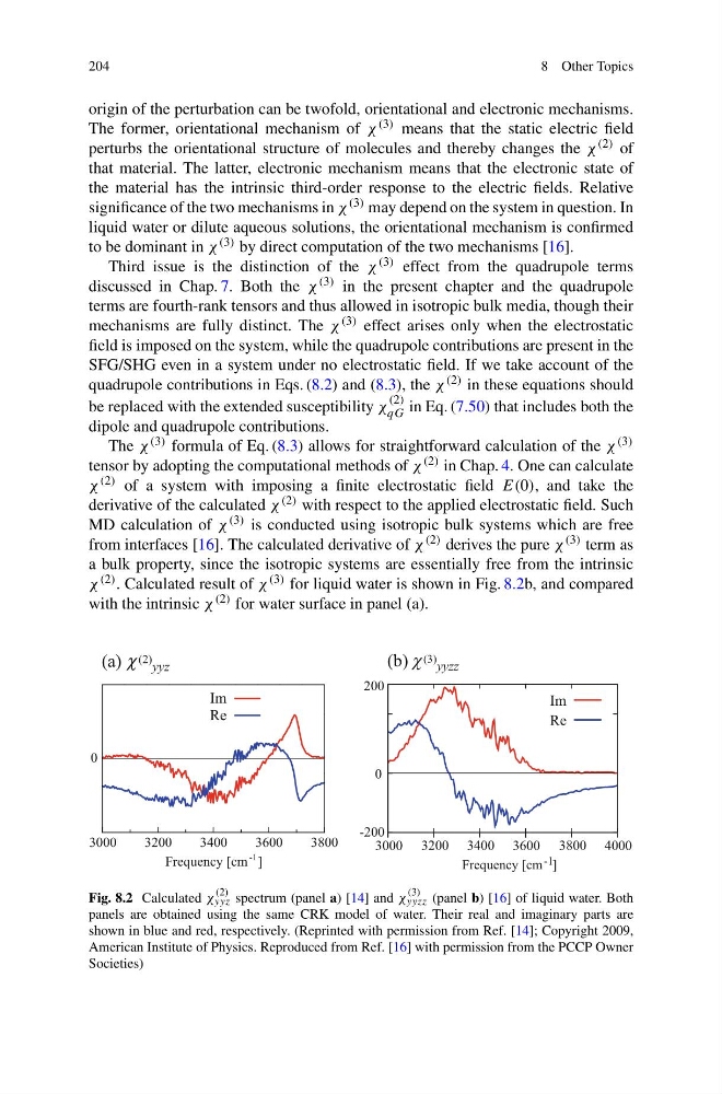
χ (2) . Calculated result of χ (3) for liquid water is shown in Fig. 8.2b, and compared
with the intrinsic χ (2) for water surface in panel (a).
-1
3000
3200
3400
3600
3800
0
(a) (2) yyz
(b) (3) yyzz
Frequency [cm ]
Im
Re
Im
Re
-1
3000 3200 3400 3600 3800
Frequency [cm ]
4000
-200
0
200
Fig. 8.2 Calculated χ
(2)
yyz spectrum (panel a) [14] and χ
(3)
yyzz (panel b) [16] of liquid water. Both
panels are obtained using the same CRK model of water. Their real and imaginary parts are
shown in blue and red, respectively. (Reprinted with permission from Ref. [14]; Copyright 2009,
American Institute of Physics. Reproduced from Ref. [16] with permission from the PCCP Owner
Societies)
8 Other Topics
origin of the perturbation can be twofold, orientational and electronic mechanisms.
The former, orientational mechanism of χ (3) means that the static electric field
perturbs the orientational structure of molecules and thereby changes the χ (2) of
that material. The latter, electronic mechanism means that the electronic state of
the material has the intrinsic third-order response to the electric fields. Relative
significance of the two mechanisms in χ (3) may depend on the system in question. In
liquid water or dilute aqueous solutions, the orientational mechanism is confirmed
to be dominant in χ (3) by direct computation of the two mechanisms [16].
Third issue is the distinction of the χ (3) effect from the quadrupole terms
discussed in Chap. 7. Both the χ (3) in the present chapter and the quadrupole
terms are fourth-rank tensors and thus allowed in isotropic bulk media, though their
mechanisms are fully distinct. The χ (3) effect arises only when the electrostatic
field is imposed on the system, while the quadrupole contributions are present in the
SFG/SHG even in a system under no electrostatic field. If we take account of the
quadrupole contributions in Eqs. (8.2) and (8.3), the χ (2) in these equations should
be replaced with the extended susceptibility χ
(2)
qG in Eq. (7.50) that includes both the
dipole and quadrupole contributions.
The χ (3) formula of Eq. (8.3) allows for straightforward calculation of the χ (3)
tensor by adopting the computational methods of χ (2) in Chap. 4. One can calculate
χ (2) of a system with imposing a finite electrostatic field E(0), and take the
derivative of the calculated χ (2) with respect to the applied electrostatic field. Such
MD calculation of χ (3) is conducted using isotropic bulk systems which are free
from interfaces [16]. The calculated derivative of χ (2) derives the pure χ (3) term as
a bulk property, since the isotropic systems are essentially free from the intrinsic
χ (2) . Calculated result of χ (3) for liquid water is shown in Fig. 8.2b, and compared
with the intrinsic χ (2) for water surface in panel (a).
-1
3000
3200
3400
3600
3800
0
(a) (2) yyz
(b) (3) yyzz
Frequency [cm ]
Im
Re
Im
Re
-1
3000 3200 3400 3600 3800
Frequency [cm ]
4000
-200
0
200
Fig. 8.2 Calculated χ
(2)
yyz spectrum (panel a) [14] and χ
(3)
yyzz (panel b) [16] of liquid water. Both
panels are obtained using the same CRK model of water. Their real and imaginary parts are
shown in blue and red, respectively. (Reprinted with permission from Ref. [14]; Copyright 2009,
American Institute of Physics. Reproduced from Ref. [16] with permission from the PCCP Owner
Societies)