

7.3 Microscopic Formulas of Quadrupolar Susceptibilities
173
+
q,r,s
α
D2
pqrs ((, ω 1 , ω 2 )E q (ω 1 )(∇E(ω 2 )) sr
(7.68)
+ · · ·
q sp (() =
q,r
α
Q
pqrs ((, ω 1 , ω 2 )E q (ω 2 )E r (ω 2 )
(7.69)
+ · · ·
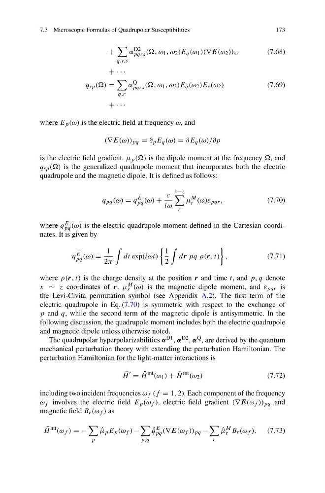
where E p (ω) is the electric field at frequency ω, and
(∇E(ω)) pq = ∂ p E q (ω) = ∂E q (ω)/∂p
is the electric field gradient. μ p (() is the dipole moment at the frequency , and
q sp (() is the generalized quadrupole moment that incorporates both the electric
quadrupole and the magnetic dipole. It is defined as follows:
q pq (ω) = q
E
pq (ω) +
c
iω
x−z
r
μ
M
r (ω)ε pqr ,
(7.70)
where q E
pq (ω) is the electric quadrupole moment defined in the Cartesian coordinates. It is given by
q
E
pq (ω) =
1
2π
dt exp(iωt)
1
2
dr pq ρ(r, t)
,
(7.71)
where ρ(r, t) is the charge density at the position r and time t, and p, q denote
x ∼ z coordinates of r. μ M
r (ω) is the magnetic dipole moment, and ε pqr is
the Levi-Civita permutation symbol (see Appendix A.2). The first term of the
electric quadrupole in Eq. (7.70) is symmetric with respect to the exchange of
p and q, while the second term of the magnetic dipole is antisymmetric. In the
following discussion, the quadrupole moment includes both the electric quadrupole
and magnetic dipole unless otherwise noted.
The quadrupolar hyperpolarizabilities α D1 , α D2 , α Q , are derived by the quantum
mechanical perturbation theory with extending the perturbation Hamiltonian. The
perturbation Hamiltonian for the light-matter interactions is
ˆ
H
= ˆ
H
int (ω 1 ) + ˆ
H
int (ω 2 )
(7.72)
including two incident frequencies ω f (f = 1, 2). Each component of the frequency
ω f involves the electric field E p (ω f ), electric field gradient (∇E(ω f )) pq and
magnetic field B r (ω f ) as
ˆ
H
int (ω f ) = −
p
ˆ
μ p E p (ω f ) −
p,q
ˆ
q
E
pq (∇E(ω f )) pq −
r
ˆ
μ
M
r B r (ω f ).
(7.73)
173
+
q,r,s
α
D2
pqrs ((, ω 1 , ω 2 )E q (ω 1 )(∇E(ω 2 )) sr
(7.68)
+ · · ·
q sp (() =
q,r
α
Q
pqrs ((, ω 1 , ω 2 )E q (ω 2 )E r (ω 2 )
(7.69)
+ · · ·
where E p (ω) is the electric field at frequency ω, and
(∇E(ω)) pq = ∂ p E q (ω) = ∂E q (ω)/∂p
is the electric field gradient. μ p (() is the dipole moment at the frequency , and
q sp (() is the generalized quadrupole moment that incorporates both the electric
quadrupole and the magnetic dipole. It is defined as follows:
q pq (ω) = q
E
pq (ω) +
c
iω
x−z
r
μ
M
r (ω)ε pqr ,
(7.70)
where q E
pq (ω) is the electric quadrupole moment defined in the Cartesian coordinates. It is given by
q
E
pq (ω) =
1
2π
dt exp(iωt)
1
2
dr pq ρ(r, t)
,
(7.71)
where ρ(r, t) is the charge density at the position r and time t, and p, q denote
x ∼ z coordinates of r. μ M
r (ω) is the magnetic dipole moment, and ε pqr is
the Levi-Civita permutation symbol (see Appendix A.2). The first term of the
electric quadrupole in Eq. (7.70) is symmetric with respect to the exchange of
p and q, while the second term of the magnetic dipole is antisymmetric. In the
following discussion, the quadrupole moment includes both the electric quadrupole
and magnetic dipole unless otherwise noted.
The quadrupolar hyperpolarizabilities α D1 , α D2 , α Q , are derived by the quantum
mechanical perturbation theory with extending the perturbation Hamiltonian. The
perturbation Hamiltonian for the light-matter interactions is
ˆ
H
= ˆ
H
int (ω 1 ) + ˆ
H
int (ω 2 )
(7.72)
including two incident frequencies ω f (f = 1, 2). Each component of the frequency
ω f involves the electric field E p (ω f ), electric field gradient (∇E(ω f )) pq and
magnetic field B r (ω f ) as
ˆ
H
int (ω f ) = −
p
ˆ
μ p E p (ω f ) −
p,q
ˆ
q
E
pq (∇E(ω f )) pq −
r
ˆ
μ
M
r B r (ω f ).
(7.73)