

158
7 Quadrupole Contributions from Interface and Bulk
dipole in response to the electric field and field gradient. A quantity which couples
with the field gradient is of quadrupolar character, as will be evident in Sect. 7.3.
The fourth line includes the induced quadrupole,
Q
(2)
0,sp (r, ,, t) ≡
q,r
χ
Q
pqrs (z, ,, ω 1 , ω 2 )E
loc
q (r, ω 1 , t)E
loc
r (r, ω 2 , t),
(7.21)
and the gradient of the quadrupole −
∂
∂s
Q
(2)
0,sp gives rise to a part of the dipole
polarization. Note that all the quadrupole terms in Eq. (7.20) are associated to spatial
gradient ∂/∂s.
We notice that the quadrupolar susceptibilities, χ D1 , χ D2 and χ Q , are non-zero in
the bulk region in contrast to the dipolar susceptibility χ D0 (see Problem 1.1). The
contrasting selection rules stem from the fact that χ D1 , χ D2 , χ Q are fourth-rank
(even-rank) tensors while χ D0 is third-rank (odd-rank). Material properties of evenrank tensors do not necessarily vanish non-centrosymmetric media for symmetry
reason. Therefore, the sum-frequency polarization P
(2)
0 (r, ,, t) in Eq. (7.20) is
induced in the bulk region (z < 0) in addition to the interface (z ≈ 0). We
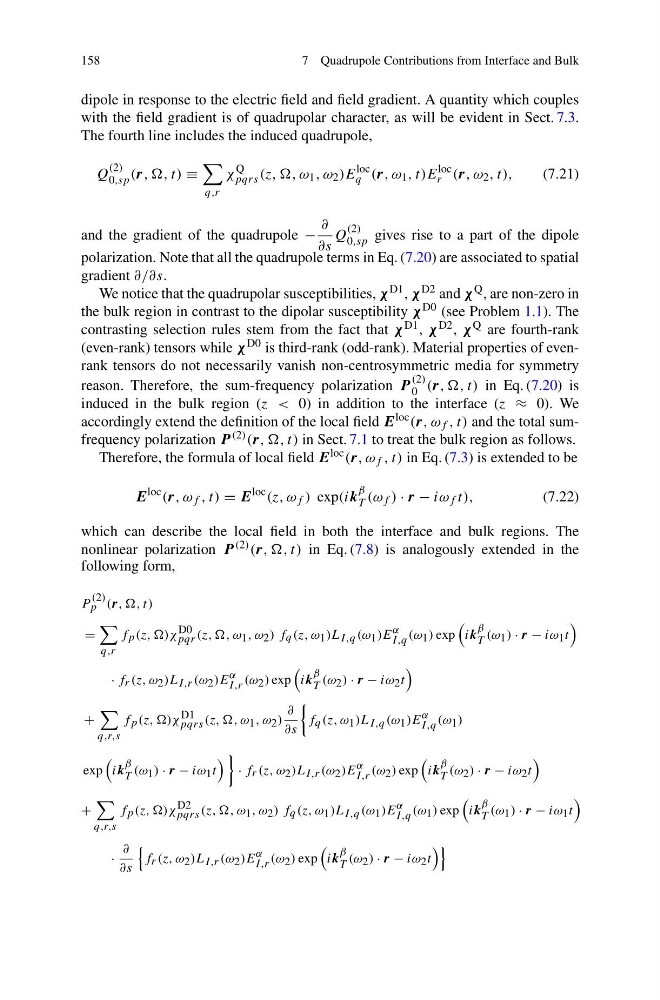
accordingly extend the definition of the local field E loc (r, ω f , t) and the total sumfrequency polarization P (2) (r, ,, t) in Sect. 7.1 to treat the bulk region as follows.
Therefore, the formula of local field E loc (r, ω f , t) in Eq. (7.3) is extended to be
E
loc (r, ω f , t) = E
loc (z, ω f ) exp(ik
β
T (ω f ) · r − iω f t),
(7.22)
which can describe the local field in both the interface and bulk regions. The
nonlinear polarization P (2) (r, ,, t) in Eq. (7.8) is analogously extended in the
following form,
P
(2)
p (r, ,, t)
=
q,r
f p (z, ,)χ D0
pqr (z, ,, ω 1 , ω 2 ) f q (z, ω 1 )L I,q (ω 1 )E α
I,q (ω 1 ) exp
ik
β
T (ω 1 ) · r − iω 1 t
· f r (z, ω 2 )L I,r (ω 2 )E α
I,r (ω 2 ) exp
ik
β
T (ω 2 ) · r − iω 2 t
+
q,r,s
f p (z, ,)χ D1
pqrs (z, ,, ω 1 , ω 2 )
∂
∂s
f q (z, ω 1 )L I,q (ω 1 )E α
I,q (ω 1 )
exp
ik
β
T (ω 1 ) · r − iω 1 t
· f r (z, ω 2 )L I,r (ω 2 )E α
I,r (ω 2 ) exp
ik
β
T (ω 2 ) · r − iω 2 t
+
q,r,s
f p (z, ,)χ D2
pqrs (z, ,, ω 1 , ω 2 ) f q (z, ω 1 )L I,q (ω 1 )E α
I,q (ω 1 ) exp
ik
β
T (ω 1 ) · r − iω 1 t
·
∂
∂s
f r (z, ω 2 )L I,r (ω 2 )E α
I,r (ω 2 ) exp
ik
β
T (ω 2 ) · r − iω 2 t
7 Quadrupole Contributions from Interface and Bulk
dipole in response to the electric field and field gradient. A quantity which couples
with the field gradient is of quadrupolar character, as will be evident in Sect. 7.3.
The fourth line includes the induced quadrupole,
Q
(2)
0,sp (r, ,, t) ≡
q,r
χ
Q
pqrs (z, ,, ω 1 , ω 2 )E
loc
q (r, ω 1 , t)E
loc
r (r, ω 2 , t),
(7.21)
and the gradient of the quadrupole −
∂
∂s
Q
(2)
0,sp gives rise to a part of the dipole
polarization. Note that all the quadrupole terms in Eq. (7.20) are associated to spatial
gradient ∂/∂s.
We notice that the quadrupolar susceptibilities, χ D1 , χ D2 and χ Q , are non-zero in
the bulk region in contrast to the dipolar susceptibility χ D0 (see Problem 1.1). The
contrasting selection rules stem from the fact that χ D1 , χ D2 , χ Q are fourth-rank
(even-rank) tensors while χ D0 is third-rank (odd-rank). Material properties of evenrank tensors do not necessarily vanish non-centrosymmetric media for symmetry
reason. Therefore, the sum-frequency polarization P
(2)
0 (r, ,, t) in Eq. (7.20) is
induced in the bulk region (z < 0) in addition to the interface (z ≈ 0). We
accordingly extend the definition of the local field E loc (r, ω f , t) and the total sumfrequency polarization P (2) (r, ,, t) in Sect. 7.1 to treat the bulk region as follows.
Therefore, the formula of local field E loc (r, ω f , t) in Eq. (7.3) is extended to be
E
loc (r, ω f , t) = E
loc (z, ω f ) exp(ik
β
T (ω f ) · r − iω f t),
(7.22)
which can describe the local field in both the interface and bulk regions. The
nonlinear polarization P (2) (r, ,, t) in Eq. (7.8) is analogously extended in the
following form,
P
(2)
p (r, ,, t)
=
q,r
f p (z, ,)χ D0
pqr (z, ,, ω 1 , ω 2 ) f q (z, ω 1 )L I,q (ω 1 )E α
I,q (ω 1 ) exp
ik
β
T (ω 1 ) · r − iω 1 t
· f r (z, ω 2 )L I,r (ω 2 )E α
I,r (ω 2 ) exp
ik
β
T (ω 2 ) · r − iω 2 t
+
q,r,s
f p (z, ,)χ D1
pqrs (z, ,, ω 1 , ω 2 )
∂
∂s
f q (z, ω 1 )L I,q (ω 1 )E α
I,q (ω 1 )
exp
ik
β
T (ω 1 ) · r − iω 1 t
· f r (z, ω 2 )L I,r (ω 2 )E α
I,r (ω 2 ) exp
ik
β
T (ω 2 ) · r − iω 2 t
+
q,r,s
f p (z, ,)χ D2
pqrs (z, ,, ω 1 , ω 2 ) f q (z, ω 1 )L I,q (ω 1 )E α
I,q (ω 1 ) exp
ik
β
T (ω 1 ) · r − iω 1 t
·
∂
∂s
f r (z, ω 2 )L I,r (ω 2 )E α
I,r (ω 2 ) exp
ik
β
T (ω 2 ) · r − iω 2 t