

98
4 Two Computational Schemes of χ (2)
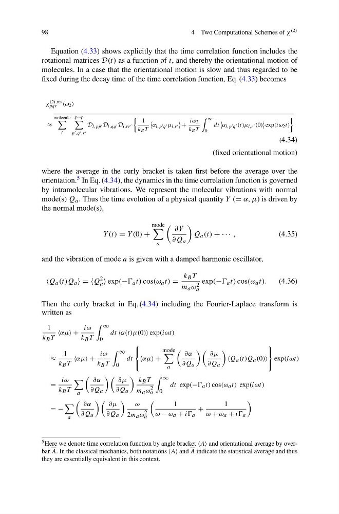
Equation (4.33) shows explicitly that the time correlation function includes the
rotational matrices D(t) as a function of t, and thereby the orientational motion of
molecules. In a case that the orientational motion is slow and thus regarded to be
fixed during the decay time of the time correlation function, Eq. (4.33) becomes
χ
(2),res
pqr (ω 2 )
≈
molecule
l
ξ ∼ζ
p ,q ,r
D l,pp D l,qq D l,rr
1
k B T
α l,p q μ l,r
+
iω 2
k B T
∞
0
dt
α l,p q (t)μ l,r (0)
exp(iω 2 t)
(4.34)
(fixed orientational motion)
where the average in the curly bracket is taken first before the average over the
orientation. 5 In Eq. (4.34), the dynamics in the time correlation function is governed
by intramolecular vibrations. We represent the molecular vibrations with normal
mode(s) Q a . Thus the time evolution of a physical quantity Y (= α, μ) is driven by
the normal mode(s),
Y (t) = Y (0) +
mode
a
∂Y
∂Q a
Q a (t) + · · · ,
(4.35)
and the vibration of mode a is given with a damped harmonic oscillator,
Q a (t)Q a = =Q
2
a exp(− a t) cos(ω a t) =
k B T
m a ω 2
a
exp(− a t) cos(ω a t).
(4.36)
Then the curly bracket in Eq. (4.34) including the Fourier-Laplace transform is
written as
1
k B T
αμ +
iω
k B T
∞
0
dt α(t)μ(0) exp(iωt)
≈
1
k B T
αμ +
iω
k B T
∞
0
dt
⎧
⎨
⎩
αμ +
mode
a
∂α
∂Q a
∂μ
∂Q a
Q a (t)Q a (0)
⎫
⎬
⎭
exp(iωt)
=
iω
k B T
a
∂α
∂Q a
∂μ
∂Q a
k B T
m a ω 2
a
∞
0
dt exp(− a t) cos(ω a t) exp(iωt)
= −
a
∂α
∂Q a
∂μ
∂Q a
ω
2m a ω 2
a
1
ω − ω a + ii a
+
1
ω + ω a + ii a
5 Here we denote time correlation function by angle bracket A and orientational average by overbar A. In the classical mechanics, both notations A and A indicate the statistical average and thus
they are essentially equivalent in this context.
4 Two Computational Schemes of χ (2)
Equation (4.33) shows explicitly that the time correlation function includes the
rotational matrices D(t) as a function of t, and thereby the orientational motion of
molecules. In a case that the orientational motion is slow and thus regarded to be
fixed during the decay time of the time correlation function, Eq. (4.33) becomes
χ
(2),res
pqr (ω 2 )
≈
molecule
l
ξ ∼ζ
p ,q ,r
D l,pp D l,qq D l,rr
1
k B T
α l,p q μ l,r
+
iω 2
k B T
∞
0
dt
α l,p q (t)μ l,r (0)
exp(iω 2 t)
(4.34)
(fixed orientational motion)
where the average in the curly bracket is taken first before the average over the
orientation. 5 In Eq. (4.34), the dynamics in the time correlation function is governed
by intramolecular vibrations. We represent the molecular vibrations with normal
mode(s) Q a . Thus the time evolution of a physical quantity Y (= α, μ) is driven by
the normal mode(s),
Y (t) = Y (0) +
mode
a
∂Y
∂Q a
Q a (t) + · · · ,
(4.35)
and the vibration of mode a is given with a damped harmonic oscillator,
Q a (t)Q a = =Q
2
a exp(− a t) cos(ω a t) =
k B T
m a ω 2
a
exp(− a t) cos(ω a t).
(4.36)
Then the curly bracket in Eq. (4.34) including the Fourier-Laplace transform is
written as
1
k B T
αμ +
iω
k B T
∞
0
dt α(t)μ(0) exp(iωt)
≈
1
k B T
αμ +
iω
k B T
∞
0
dt
⎧
⎨
⎩
αμ +
mode
a
∂α
∂Q a
∂μ
∂Q a
Q a (t)Q a (0)
⎫
⎬
⎭
exp(iωt)
=
iω
k B T
a
∂α
∂Q a
∂μ
∂Q a
k B T
m a ω 2
a
∞
0
dt exp(− a t) cos(ω a t) exp(iωt)
= −
a
∂α
∂Q a
∂μ
∂Q a
ω
2m a ω 2
a
1
ω − ω a + ii a
+
1
ω + ω a + ii a
5 Here we denote time correlation function by angle bracket A and orientational average by overbar A. In the classical mechanics, both notations A and A indicate the statistical average and thus
they are essentially equivalent in this context.