

4.4 Motional Effect on χ (2)
97
4.4.1 Relation of Two χ (2) Models
For this purpose, we clarify the relation and difference of the two χ (2) modeling on
the basis of energy representation and time-dependent representation. The energy
representation model of χ (2) in Eqs. (4.3) and (4.4) can be derived from the timedependent representation in Eq. (4.29) with employing some assumptions.
Since Eq. (4.29) refers to the nonlinear susceptibility χ (2) of the whole interface
system, α and μ in this equation also stand for the polarizability and dipole of the
whole system. Thus α and μ of the whole interface system are expressed as the sum
of molecular quantities,
α pq ≈
molecule
l
ξ ∼ζ
p
ξ ∼ζ
q
D l,pp D l,qq α l,p q ,
(4.31)
μ r ≈
molecule
k
ξ ∼ζ
r
D k,rr μ k,r ,
(4.32)
where α l,p q and μ k,p denote the polarizability tensor of l-th molecule and the
dipole vector of k-th molecule, respectively, in the molecule-fixed coordinates. We
note that Eqs. (4.31) and (4.32) are regarded as a crude approximation to neglect the
local field effect. The local field effect will be discussed in details in Chap. 5, and
thereby the above formulas will be refined in that chapter.
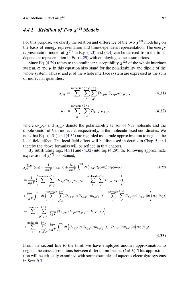
By substituting Eqs. (4.31) and (4.32) into Eq. (4.29), the following approximate
expression of χ (2) is obtained,
χ
(2),res
pqr (ω 2 ) =
1
k B T
α pq μ r +
iω 2
k B T
∞
0
dt
α pq (t)μ r (0)
exp(iω 2 t)
(4.29)
≈
1
k B T
molecule
l
ξ ∼ζ
p ,q
D l,pp D l,qq α l,p q ·
molecule
k
ξ ∼ζ
r
D k,rr μ k,r
+
iω 2
k B T
∞
0
dt
molecule
l
ξ ∼ζ
p ,q
D l,pp (t)D l,qq (t)α l,p q (t) ·
molecule
k
ξ ∼ζ
r
D k,rr (0)μ k,r (0)
exp(iω 2 t)
≈
molecule
l
ξ ∼ζ
p ,q ,r
1
k B T
D l,pp D l,qq α l,p q · D l,rr μ l,r
+
molecule
l
ξ ∼ζ
p ,q ,r
iω 2
k B T
∞
0
dt
D l,pp (t)D l,qq (t)α l,p q (t) · D l,rr (0)μ l,r (0)
exp(iω 2 t).
(4.33)
From the second line to the third, we have employed another approximation to
neglect the cross correlations between different molecules (l = k). This approximation will be critically examined with some examples of aqueous electrolyte systems
in Sect. 9.3.
97
4.4.1 Relation of Two χ (2) Models
For this purpose, we clarify the relation and difference of the two χ (2) modeling on
the basis of energy representation and time-dependent representation. The energy
representation model of χ (2) in Eqs. (4.3) and (4.4) can be derived from the timedependent representation in Eq. (4.29) with employing some assumptions.
Since Eq. (4.29) refers to the nonlinear susceptibility χ (2) of the whole interface
system, α and μ in this equation also stand for the polarizability and dipole of the
whole system. Thus α and μ of the whole interface system are expressed as the sum
of molecular quantities,
α pq ≈
molecule
l
ξ ∼ζ
p
ξ ∼ζ
q
D l,pp D l,qq α l,p q ,
(4.31)
μ r ≈
molecule
k
ξ ∼ζ
r
D k,rr μ k,r ,
(4.32)
where α l,p q and μ k,p denote the polarizability tensor of l-th molecule and the
dipole vector of k-th molecule, respectively, in the molecule-fixed coordinates. We
note that Eqs. (4.31) and (4.32) are regarded as a crude approximation to neglect the
local field effect. The local field effect will be discussed in details in Chap. 5, and
thereby the above formulas will be refined in that chapter.
By substituting Eqs. (4.31) and (4.32) into Eq. (4.29), the following approximate
expression of χ (2) is obtained,
χ
(2),res
pqr (ω 2 ) =
1
k B T
α pq μ r +
iω 2
k B T
∞
0
dt
α pq (t)μ r (0)
exp(iω 2 t)
(4.29)
≈
1
k B T
molecule
l
ξ ∼ζ
p ,q
D l,pp D l,qq α l,p q ·
molecule
k
ξ ∼ζ
r
D k,rr μ k,r
+
iω 2
k B T
∞
0
dt
molecule
l
ξ ∼ζ
p ,q
D l,pp (t)D l,qq (t)α l,p q (t) ·
molecule
k
ξ ∼ζ
r
D k,rr (0)μ k,r (0)
exp(iω 2 t)
≈
molecule
l
ξ ∼ζ
p ,q ,r
1
k B T
D l,pp D l,qq α l,p q · D l,rr μ l,r
+
molecule
l
ξ ∼ζ
p ,q ,r
iω 2
k B T
∞
0
dt
D l,pp (t)D l,qq (t)α l,p q (t) · D l,rr (0)μ l,r (0)
exp(iω 2 t).
(4.33)
From the second line to the third, we have employed another approximation to
neglect the cross correlations between different molecules (l = k). This approximation will be critically examined with some examples of aqueous electrolyte systems
in Sect. 9.3.