

K. Jagiełło et al.
18
Centring the data is the linear transformation performs to make all variables
coincide with the beginning of the coordinate system. It is done by subtracting from
each value x ij of data organized into matrix X corresponding mean value of jth variable to obtain new matrix X′, according to formula [1]:
′ =
−
x
x
ij
ij
j
µ
(2.2)
the autoscaling is made by diving by centered data by the standard deviation of the
jth variables according to formula (2.2). As a result, we obtained the normalized
matrix Z [2]:
z
x
ij
ij
j
j
=
− µ
σ
(2.3)
where:
x ij
molar extinction coefficient for the i-th wavelength of the j-th spectrum
µ j
the average value of the molar extinction coefficients of the j-th spectrum
σ j
standard deviation of the molar extinction coefficients of the j-th spectrum.
Spectrum after standardization can be treated as a vector of unit length. A set of
spectra creates a bunch of vectors which have common origin in the k-dimensional
hyperspace, where k is the number of spectral forms present in the analyzed samples. A bunch of vectors for recorded spectra is limited by vectors representing the
spectra of pure ingredients. An example for two component mixture (k = 2) is shown
in Fig. 2.2.
2.2.2 Internal Order of a Matrix and Number of Variety Sources
the Principal Component Analysis (PCA) [6] is a special example of projection
pursuit techniques, in which variance is used as a projection index. PCA is mainly
used for modeling, compressing and visualizing multidimensional data [7–10].
Application PCA in the relationship analysis involves two basic tasks: graphical
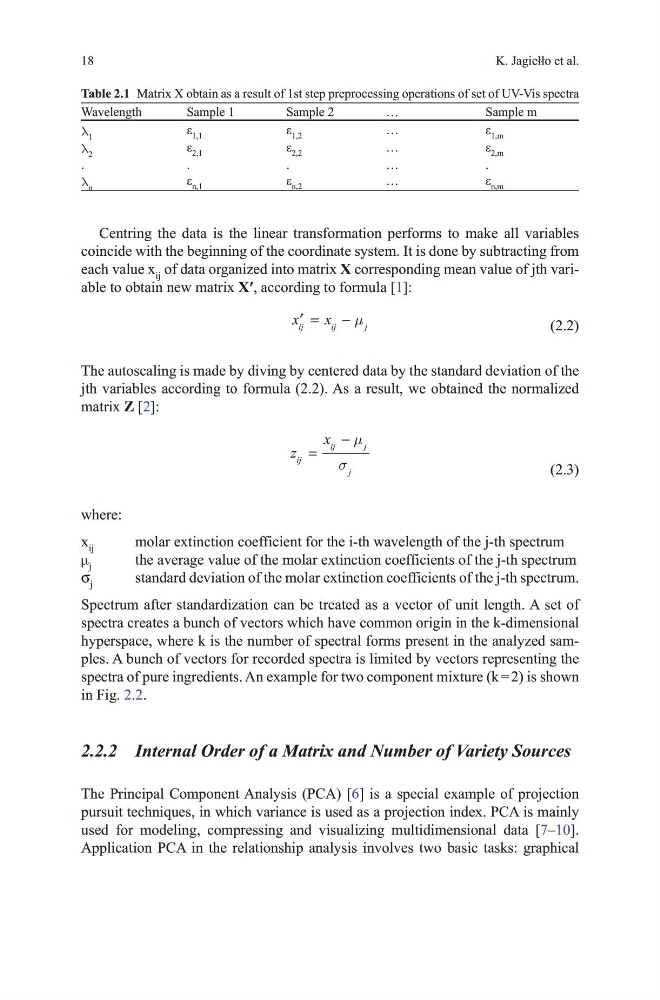
Table 2.1 matrix X obtain as a result of 1st step preprocessing operations of set of uv-vis spectra
Wavelength
Sample 1
Sample 2
…
Sample m
λ 1
ε 1,1
ε 1,2
…
ε 1,m
λ 2
ε 2,1
ε 2,2
…
ε 2,m
.
.
.
…
.
λ n
ε n,1
ε n,2
…
ε n,m
18
Centring the data is the linear transformation performs to make all variables
coincide with the beginning of the coordinate system. It is done by subtracting from
each value x ij of data organized into matrix X corresponding mean value of jth variable to obtain new matrix X′, according to formula [1]:
′ =
−
x
x
ij
ij
j
µ
(2.2)
the autoscaling is made by diving by centered data by the standard deviation of the
jth variables according to formula (2.2). As a result, we obtained the normalized
matrix Z [2]:
z
x
ij
ij
j
j
=
− µ
σ
(2.3)
where:
x ij
molar extinction coefficient for the i-th wavelength of the j-th spectrum
µ j
the average value of the molar extinction coefficients of the j-th spectrum
σ j
standard deviation of the molar extinction coefficients of the j-th spectrum.
Spectrum after standardization can be treated as a vector of unit length. A set of
spectra creates a bunch of vectors which have common origin in the k-dimensional
hyperspace, where k is the number of spectral forms present in the analyzed samples. A bunch of vectors for recorded spectra is limited by vectors representing the
spectra of pure ingredients. An example for two component mixture (k = 2) is shown
in Fig. 2.2.
2.2.2 Internal Order of a Matrix and Number of Variety Sources
the Principal Component Analysis (PCA) [6] is a special example of projection
pursuit techniques, in which variance is used as a projection index. PCA is mainly
used for modeling, compressing and visualizing multidimensional data [7–10].
Application PCA in the relationship analysis involves two basic tasks: graphical
Table 2.1 matrix X obtain as a result of 1st step preprocessing operations of set of uv-vis spectra
Wavelength
Sample 1
Sample 2
…
Sample m
λ 1
ε 1,1
ε 1,2
…
ε 1,m
λ 2
ε 2,1
ε 2,2
…
ε 2,m
.
.
.
…
.
λ n
ε n,1
ε n,2
…
ε n,m