

2 Integrating Optical Spectroscopy and Chemometric Methods
19
presentation of the dimensional dependence and reducing the dimensionality of
the problem. In this technique, set of correlation coefficient between variables in
multivariate space might be transformed to equivalent set of orthogonal factors.
the principal components are new orthogonal variables (which are expressed as
a linear combination of original variables) and they maximized description of the
data variance.
the PCA analysis allows to determine the internal dimension of the matrix of
the standardized spectra. this dimension is equal to the number of spectral forms
presented in the samples. If the spectra of individual species are not excessively correlated, it is equal to the number of significant principal components of this matrix.
unfortunately, when the spectral forms have very similar spectra, as is usual in the
case of aggregation, the analysis of the residual spectra have to be used to determine
the number of spectral species in the samples [3, 4].
the principal components and their loadings permit to complete reconstruction
of the standardized spectra matrix according to the equation:
Z
P L
nm
nm nm
=
(2.4)
where:
P nm
matrix of m principal components,
L nm
matrix of loadings.
If in the spectra reconstruction we use only j first principal components we obtain
following relationship:
Z
P L
E
nm
nj jm
j
=
+
( )
(2.5)
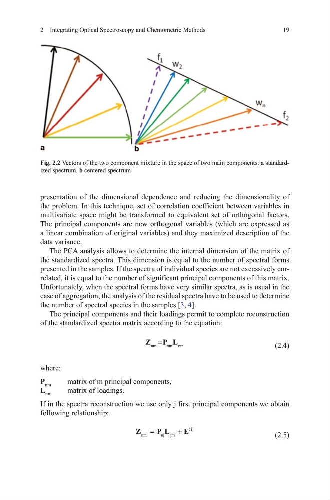
Fig. 2.2 vectors of the two component mixture in the space of two main components: a standardized spectrum. b centered spectrum
19
presentation of the dimensional dependence and reducing the dimensionality of
the problem. In this technique, set of correlation coefficient between variables in
multivariate space might be transformed to equivalent set of orthogonal factors.
the principal components are new orthogonal variables (which are expressed as
a linear combination of original variables) and they maximized description of the
data variance.
the PCA analysis allows to determine the internal dimension of the matrix of
the standardized spectra. this dimension is equal to the number of spectral forms
presented in the samples. If the spectra of individual species are not excessively correlated, it is equal to the number of significant principal components of this matrix.
unfortunately, when the spectral forms have very similar spectra, as is usual in the
case of aggregation, the analysis of the residual spectra have to be used to determine
the number of spectral species in the samples [3, 4].
the principal components and their loadings permit to complete reconstruction
of the standardized spectra matrix according to the equation:
Z
P L
nm
nm nm
=
(2.4)
where:
P nm
matrix of m principal components,
L nm
matrix of loadings.
If in the spectra reconstruction we use only j first principal components we obtain
following relationship:
Z
P L
E
nm
nj jm
j
=
+
( )
(2.5)
Fig. 2.2 vectors of the two component mixture in the space of two main components: a standardized spectrum. b centered spectrum