

1 Nanoplasmonics: From Present into Future
45
10
20
30
10
20
30
0
10
20
30
10
20
30
0
10
20
30
10
20
30
0
10
20
30
10
20
30
0
10
20
30
10
20
30
0
10
20
30
10
20
30
0
10
20
30
10
20
30
0
10
20
30
10
20
30
0
G(20,9)
H(24,11)
F(18,7)
E(9,7)
C(7,14)
D(7,10)
B(7,16)
A(11,22)
2×10 6
6×10 7
3×10 7
1×10 7
5×10 6
z
x
z
x
z
x
z
x
z
x
z
x
z
x
4×10 6
2×10 4
4×10 4
5×10 3
1×10 4
5×10 4
1×10 5
z
x
1×10 8
5×10 7
1×10 6
5×10 5
<
>
I 2 >
<
>
I 2 >
<
>
I 2 >
(a)
(b)
(c)
(d)
(e)
(f)
(g)
(h)
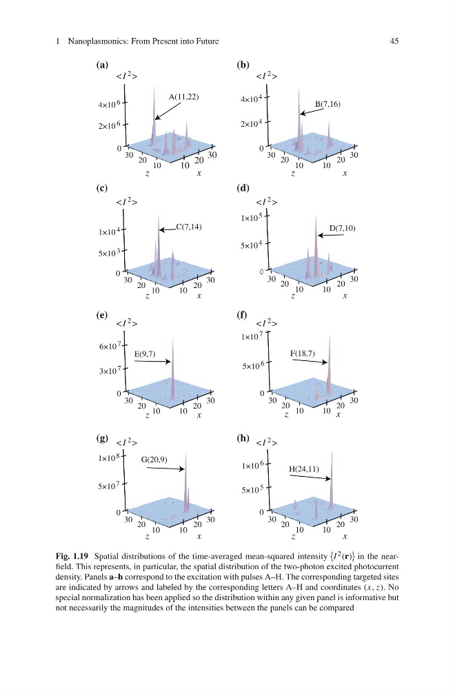
Fig. 1.19 Spatial distributions of the time-averaged mean-squared intensity
I 2 (r)
in the nearfield. This represents, in particular, the spatial distribution of the two-photon excited photocurrent
density. Panels a–h correspond to the excitation with pulses A–H. The corresponding targeted sites
are indicated by arrows and labeled by the corresponding letters A–H and coordinates (x, z). No
special normalization has been applied so the distribution within any given panel is informative but
not necessarily the magnitudes of the intensities between the panels can be compared
45
10
20
30
10
20
30
0
10
20
30
10
20
30
0
10
20
30
10
20
30
0
10
20
30
10
20
30
0
10
20
30
10
20
30
0
10
20
30
10
20
30
0
10
20
30
10
20
30
0
10
20
30
10
20
30
0
G(20,9)
H(24,11)
F(18,7)
E(9,7)
C(7,14)
D(7,10)
B(7,16)
A(11,22)
2×10 6
6×10 7
3×10 7
1×10 7
5×10 6
z
x
z
x
z
x
z
x
z
x
z
x
z
x
4×10 6
2×10 4
4×10 4
5×10 3
1×10 4
5×10 4
1×10 5
z
x
1×10 8
5×10 7
1×10 6
5×10 5
<
>
I 2 >
<
>
I 2 >
<
>
I 2 >
(a)
(b)
(c)
(d)
(e)
(f)
(g)
(h)
Fig. 1.19 Spatial distributions of the time-averaged mean-squared intensity
I 2 (r)
in the nearfield. This represents, in particular, the spatial distribution of the two-photon excited photocurrent
density. Panels a–h correspond to the excitation with pulses A–H. The corresponding targeted sites
are indicated by arrows and labeled by the corresponding letters A–H and coordinates (x, z). No
special normalization has been applied so the distribution within any given panel is informative but
not necessarily the magnitudes of the intensities between the panels can be compared