

44
M. I. Stockman
0
100 200 300
0
0
100 200 300
0
0
100 200 300
0
0
100 200 300
0
0
100 200 300
0
0
100 200 300
0
0
100 200 300
0
0
100 200 300
0
1×10 4
2×10 4
2×10 3
500
4×10 4
8×10 4
4×10 4
8×10 4
2×10 3
2×10 3
4×10 3
4×10 3
8×10 3
1×10 3
1×10 3
(e)
(a)
(h)
(g)
(f)
(b)
(c)
(d)
C
B
A
D
F
H
G
E
I
I
I
I
I
I
I
I
t (fs)
t (fs)
t (fs)
t (fs)
t (fs)
t (fs)
t (fs)
t (fs)
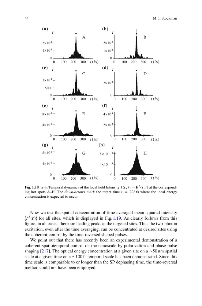
Fig. 1.18 a–h Temporal dynamics of the local field Intensity I (r, t) = E 2 (r, t) at the corresponding hot spots A–H. The down-arrows mark the target time t = 228 fs where the local energy
concentration is expected to occur
Now we test the spatial concentration of time-averaged mean-squared intensity
I 2 (r)
for all sites, which is displayed in Fig. 1.19. As clearly follows from this
figure, in all cases, there are leading peaks at the targeted sites. Thus the two-photon
excitation, even after the time averaging, can be concentrated at desired sites using
the coherent-control by the time-reversed shaped pulses.
We point out that there has recently been an experimental demonstration of a
coherent spatiotemporal control on the nanoscale by polarization and phase pulse
shaping [217]. The optical energy concentration at a given site on a ∼50 nm spatial
scale at a given time on a ∼100 fs temporal scale has been demonstrated. Since this
time scale is comparable to or longer than the SP dephasing time, the time-reversal
method could not have been employed.
M. I. Stockman
0
100 200 300
0
0
100 200 300
0
0
100 200 300
0
0
100 200 300
0
0
100 200 300
0
0
100 200 300
0
0
100 200 300
0
0
100 200 300
0
1×10 4
2×10 4
2×10 3
500
4×10 4
8×10 4
4×10 4
8×10 4
2×10 3
2×10 3
4×10 3
4×10 3
8×10 3
1×10 3
1×10 3
(e)
(a)
(h)
(g)
(f)
(b)
(c)
(d)
C
B
A
D
F
H
G
E
I
I
I
I
I
I
I
I
t (fs)
t (fs)
t (fs)
t (fs)
t (fs)
t (fs)
t (fs)
t (fs)
Fig. 1.18 a–h Temporal dynamics of the local field Intensity I (r, t) = E 2 (r, t) at the corresponding hot spots A–H. The down-arrows mark the target time t = 228 fs where the local energy
concentration is expected to occur
Now we test the spatial concentration of time-averaged mean-squared intensity
I 2 (r)
for all sites, which is displayed in Fig. 1.19. As clearly follows from this
figure, in all cases, there are leading peaks at the targeted sites. Thus the two-photon
excitation, even after the time averaging, can be concentrated at desired sites using
the coherent-control by the time-reversed shaped pulses.
We point out that there has recently been an experimental demonstration of a
coherent spatiotemporal control on the nanoscale by polarization and phase pulse
shaping [217]. The optical energy concentration at a given site on a ∼50 nm spatial
scale at a given time on a ∼100 fs temporal scale has been demonstrated. Since this
time scale is comparable to or longer than the SP dephasing time, the time-reversal
method could not have been employed.