

15 Cooperative Effects in Plasmonics
533
15.1.3 Radiated Energy of an Ensemble of Dipoles
Near Nanoparticle
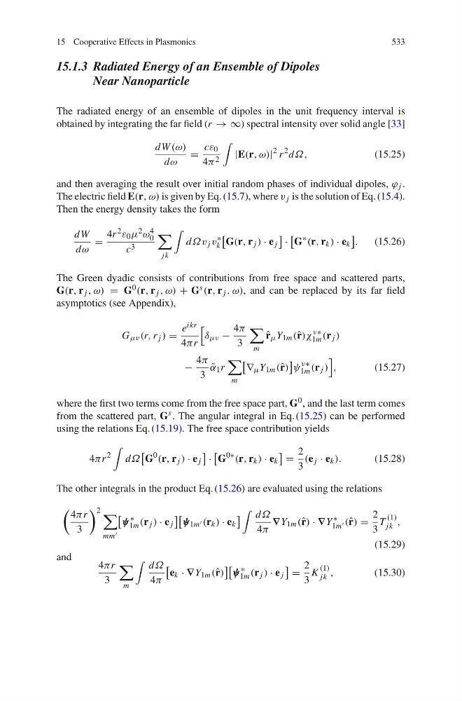
The radiated energy of an ensemble of dipoles in the unit frequency interval is
obtained by integrating the far field (r → ∞) spectral intensity over solid angle [33]
dW (ω)
dω
=
cε 0
4π 2
|E(r, ω)|
2 r
2 dΩ,
(15.25)
and then averaging the result over initial random phases of individual dipoles, ϕ j .
The electric field E(r, ω) is given by Eq. (15.7), where v j is the solution of Eq. (15.4).
Then the energy density takes the form
dW
dω
=
4r 2 ε 0 μ 2 ω 4
0
c 3
jk
dΩv j v
∗
k
G(r, r j ) · e j
·
G
∗
(r, r k ) · e k
.
(15.26)
The Green dyadic consists of contributions from free space and scattered parts,
G(r, r j , ω) = G 0 (r, r j , ω) + G s (r, r j , ω), and can be replaced by its far field
asymptotics (see Appendix),
G μν (r, r j ) =
e ikr
4πr
δ μν −
4π
3
m
ˆ
r μ Y 1m (ˆ r)χ
ν∗
1m (r j )
−
4π
3
˜
α 1 r
m
∞ μ Y 1m (ˆ r)
ψ
ν∗
1m (r j )
,
(15.27)
where the first two terms come from the free space part, G 0 , and the last term comes
from the scattered part, G s . The angular integral in Eq. (15.25) can be performed
using the relations Eq. (15.19). The free space contribution yields
4πr
2
dΩ
G
0
(r, r j ) · e j
·
G
0∗
(r, r k ) · e k
=
2
3
(e j · e k ).
(15.28)
The other integrals in the product Eq. (15.26) are evaluated using the relations
4πr
3
2
mm √
ψ
∗
1m (r j ) · e j
ψ 1m √ (r k ) · e k
dΩ
4π
∇Y 1m (ˆ r) · ∇Y
∗
1m √ (ˆ r) =
2
3
T
(1)
jk ,
(15.29)
and
4πr
3
m
dΩ
4π
e k · ∇Y 1m (ˆ r)
ψ
∗
1m (r j ) · e j
=
2
3
K
(1)
jk ,
(15.30)
533
15.1.3 Radiated Energy of an Ensemble of Dipoles
Near Nanoparticle
The radiated energy of an ensemble of dipoles in the unit frequency interval is
obtained by integrating the far field (r → ∞) spectral intensity over solid angle [33]
dW (ω)
dω
=
cε 0
4π 2
|E(r, ω)|
2 r
2 dΩ,
(15.25)
and then averaging the result over initial random phases of individual dipoles, ϕ j .
The electric field E(r, ω) is given by Eq. (15.7), where v j is the solution of Eq. (15.4).
Then the energy density takes the form
dW
dω
=
4r 2 ε 0 μ 2 ω 4
0
c 3
jk
dΩv j v
∗
k
G(r, r j ) · e j
·
G
∗
(r, r k ) · e k
.
(15.26)
The Green dyadic consists of contributions from free space and scattered parts,
G(r, r j , ω) = G 0 (r, r j , ω) + G s (r, r j , ω), and can be replaced by its far field
asymptotics (see Appendix),
G μν (r, r j ) =
e ikr
4πr
δ μν −
4π
3
m
ˆ
r μ Y 1m (ˆ r)χ
ν∗
1m (r j )
−
4π
3
˜
α 1 r
m
∞ μ Y 1m (ˆ r)
ψ
ν∗
1m (r j )
,
(15.27)
where the first two terms come from the free space part, G 0 , and the last term comes
from the scattered part, G s . The angular integral in Eq. (15.25) can be performed
using the relations Eq. (15.19). The free space contribution yields
4πr
2
dΩ
G
0
(r, r j ) · e j
·
G
0∗
(r, r k ) · e k
=
2
3
(e j · e k ).
(15.28)
The other integrals in the product Eq. (15.26) are evaluated using the relations
4πr
3
2
mm √
ψ
∗
1m (r j ) · e j
ψ 1m √ (r k ) · e k
dΩ
4π
∇Y 1m (ˆ r) · ∇Y
∗
1m √ (ˆ r) =
2
3
T
(1)
jk ,
(15.29)
and
4πr
3
m
dΩ
4π
e k · ∇Y 1m (ˆ r)
ψ
∗
1m (r j ) · e j
=
2
3
K
(1)
jk ,
(15.30)