

530
V. N. Pustovit and T. V. Shahbazyan
where G(r, r √ , ω) is the electric field Green diadic in the presence of NP. From
Eq. (15.4), for photon frequency close to dipoles frequency, ω ∈ ω 0 , we obtain a
coupled system of equations for normalized displacements,
k
(ω 0 − ω)δ jk + Σ jk
v k =
−i
2
e
−iϕ j ,
(15.8)
where Σ jk = Δ jk −
i
2 Γ jk is the complex self-energy matrix, given by
Σ jk (ω) = −
2πq 2 ω 0
mc 2 e j · G(r j , r k ; ω) · e k .
(15.9)
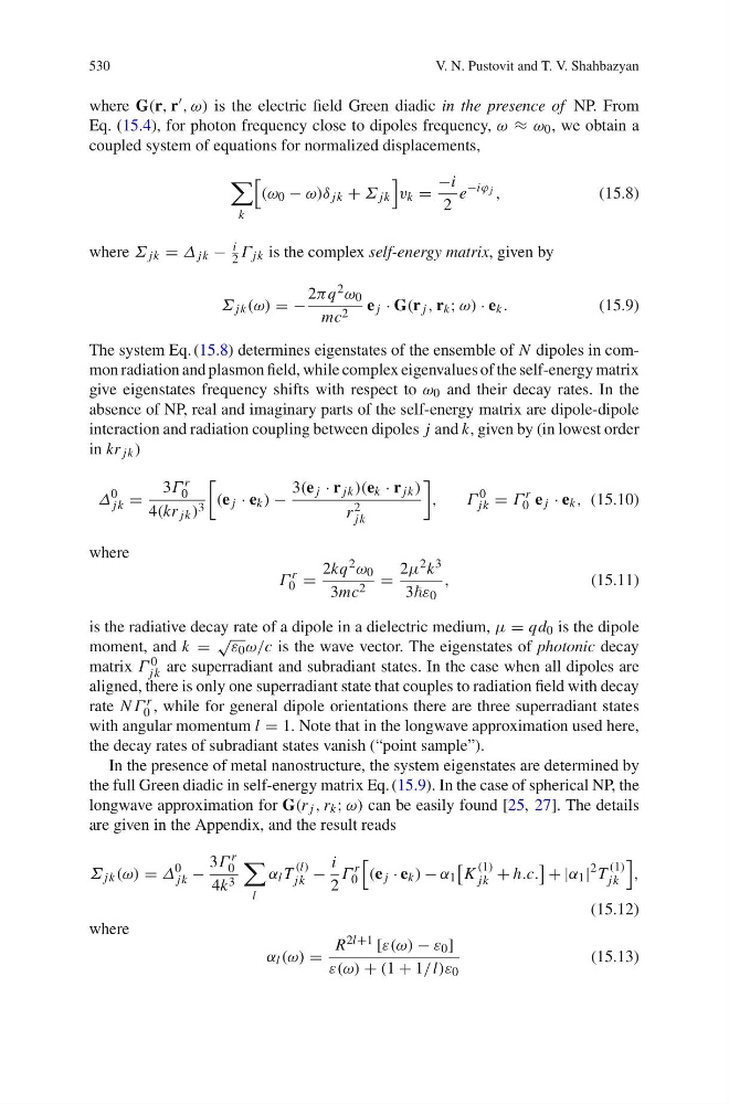
The system Eq. (15.8) determines eigenstates of the ensemble of N dipoles in common radiation and plasmon field, while complex eigenvalues of the self-energy matrix
give eigenstates frequency shifts with respect to ω 0 and their decay rates. In the
absence of NP, real and imaginary parts of the self-energy matrix are dipole-dipole
interaction and radiation coupling between dipoles j and k, given by (in lowest order
in kr jk )
Δ
0
jk =
3Γ r
0
4(kr jk ) 3
(e j · e k ) −
3(e j · r jk )(e k · r jk )
r 2
jk
,
Γ
0
jk = Γ
r
0 e j · e k , (15.10)
where
Γ
r
0 =
2kq 2 ω 0
3mc 2 =
2μ 2 k 3
3ε 0
,
(15.11)
is the radiative decay rate of a dipole in a dielectric medium, μ = qd 0 is the dipole
moment, and k =
≥
ε 0 ω/c is the wave vector. The eigenstates of photonic decay
matrix Γ 0
jk are superradiant and subradiant states. In the case when all dipoles are
aligned, there is only one superradiant state that couples to radiation field with decay
rate N Γ r
0 , while for general dipole orientations there are three superradiant states
with angular momentum l = 1. Note that in the longwave approximation used here,
the decay rates of subradiant states vanish (“point sample”).
In the presence of metal nanostructure, the system eigenstates are determined by
the full Green diadic in self-energy matrix Eq. (15.9). In the case of spherical NP, the
longwave approximation for G(r j , r k ; ω) can be easily found [25, 27]. The details
are given in the Appendix, and the result reads
Σ jk (ω) = Δ
0
jk −
3Γ r
0
4k 3
l
α l T
(l)
jk −
i
2
Γ
r
0
(e j · e k ) − α 1
K
(1)
jk + h.c.
+ |α 1 |
2 T
(1)
jk
,
(15.12)
where
α l (ω) =
R 2l+1 [ε(ω) − ε 0 ]
ε(ω) + (1 + 1/l)ε 0
(15.13)
V. N. Pustovit and T. V. Shahbazyan
where G(r, r √ , ω) is the electric field Green diadic in the presence of NP. From
Eq. (15.4), for photon frequency close to dipoles frequency, ω ∈ ω 0 , we obtain a
coupled system of equations for normalized displacements,
k
(ω 0 − ω)δ jk + Σ jk
v k =
−i
2
e
−iϕ j ,
(15.8)
where Σ jk = Δ jk −
i
2 Γ jk is the complex self-energy matrix, given by
Σ jk (ω) = −
2πq 2 ω 0
mc 2 e j · G(r j , r k ; ω) · e k .
(15.9)
The system Eq. (15.8) determines eigenstates of the ensemble of N dipoles in common radiation and plasmon field, while complex eigenvalues of the self-energy matrix
give eigenstates frequency shifts with respect to ω 0 and their decay rates. In the
absence of NP, real and imaginary parts of the self-energy matrix are dipole-dipole
interaction and radiation coupling between dipoles j and k, given by (in lowest order
in kr jk )
Δ
0
jk =
3Γ r
0
4(kr jk ) 3
(e j · e k ) −
3(e j · r jk )(e k · r jk )
r 2
jk
,
Γ
0
jk = Γ
r
0 e j · e k , (15.10)
where
Γ
r
0 =
2kq 2 ω 0
3mc 2 =
2μ 2 k 3
3ε 0
,
(15.11)
is the radiative decay rate of a dipole in a dielectric medium, μ = qd 0 is the dipole
moment, and k =
≥
ε 0 ω/c is the wave vector. The eigenstates of photonic decay
matrix Γ 0
jk are superradiant and subradiant states. In the case when all dipoles are
aligned, there is only one superradiant state that couples to radiation field with decay
rate N Γ r
0 , while for general dipole orientations there are three superradiant states
with angular momentum l = 1. Note that in the longwave approximation used here,
the decay rates of subradiant states vanish (“point sample”).
In the presence of metal nanostructure, the system eigenstates are determined by
the full Green diadic in self-energy matrix Eq. (15.9). In the case of spherical NP, the
longwave approximation for G(r j , r k ; ω) can be easily found [25, 27]. The details
are given in the Appendix, and the result reads
Σ jk (ω) = Δ
0
jk −
3Γ r
0
4k 3
l
α l T
(l)
jk −
i
2
Γ
r
0
(e j · e k ) − α 1
K
(1)
jk + h.c.
+ |α 1 |
2 T
(1)
jk
,
(15.12)
where
α l (ω) =
R 2l+1 [ε(ω) − ε 0 ]
ε(ω) + (1 + 1/l)ε 0
(15.13)