

15 Cooperative Effects in Plasmonics
529
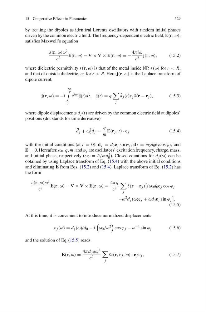
by treating the dipoles as identical Lorentz oscillators with random initial phases
driven by the common electric field. The frequency-dependent electric field, E(r, ω),
satisfies Maxwell’s equation
ε(r, ω)ω 2
c 2
E(r, ω) − ∇ × ∇ × E(r, ω) = −
4πiω
c 2 j(r, ω),
(15.2)
where dielectric permittivity ε(r, ω) is that of the metal inside NP, ε(ω) for r < R,
and that of outside dielectric, ε 0 for r > R. Here j(r, ω) is the Laplace transform of
dipole current,
j(r, ω) = −i
∞
0
e
iωt j(t)dt, j(t) = q
j
˙
d j (t)e j δ(r − r j ),
(15.3)
where dipole displacements d j (t) are driven by the common electric field at dipoles’
positions (dot stands for time derivative)
¨
d j + ω
2
0 d j =
q
m
E(r j , t) · e j
(15.4)
with the initial conditions (at t = 0): d j = d 0 e j sin ϕ j , ˙
d j = ω 0 d 0 e j cos ϕ j , and
E = 0. Hereafter, ω 0 , q, m, and ϕ j are oscillators’ excitation frequency, charge, mass,
and initial phase, respectively (ω 0 = /md 2
0 ). Closed equations for d j (ω) can be
obtained by using Laplace transform of Eq. (15.4) with the above initial conditions
and eliminating E from Eqs. (15.2) and (15.4). Laplace transform of Eq. (15.2) has
the form
ε(r, ω)ω 2
c 2
E(r, ω) − ∇ × ∇ × E(r, ω) =
4πq
c 2
j
δ(r − r j )
iω 0 d 0 e j cos ϕ j
−ω
2 d j (ω)e j + ωd 0 e j sin ϕ j
.
(15.5)
At this time, it is convenient to introduce normalized displacements
v j (ω) = d j (ω)/d 0 − i
ω 0 /ω
2
cos ϕ j − ω
−1 sin ϕ j
(15.6)
and the solution of Eq. (15.5) reads
E(r, ω) =
4π d 0 qω 2
c 2
j
G(r, r j , ω) · e j v j ,
(15.7)
529
by treating the dipoles as identical Lorentz oscillators with random initial phases
driven by the common electric field. The frequency-dependent electric field, E(r, ω),
satisfies Maxwell’s equation
ε(r, ω)ω 2
c 2
E(r, ω) − ∇ × ∇ × E(r, ω) = −
4πiω
c 2 j(r, ω),
(15.2)
where dielectric permittivity ε(r, ω) is that of the metal inside NP, ε(ω) for r < R,
and that of outside dielectric, ε 0 for r > R. Here j(r, ω) is the Laplace transform of
dipole current,
j(r, ω) = −i
∞
0
e
iωt j(t)dt, j(t) = q
j
˙
d j (t)e j δ(r − r j ),
(15.3)
where dipole displacements d j (t) are driven by the common electric field at dipoles’
positions (dot stands for time derivative)
¨
d j + ω
2
0 d j =
q
m
E(r j , t) · e j
(15.4)
with the initial conditions (at t = 0): d j = d 0 e j sin ϕ j , ˙
d j = ω 0 d 0 e j cos ϕ j , and
E = 0. Hereafter, ω 0 , q, m, and ϕ j are oscillators’ excitation frequency, charge, mass,
and initial phase, respectively (ω 0 = /md 2
0 ). Closed equations for d j (ω) can be
obtained by using Laplace transform of Eq. (15.4) with the above initial conditions
and eliminating E from Eqs. (15.2) and (15.4). Laplace transform of Eq. (15.2) has
the form
ε(r, ω)ω 2
c 2
E(r, ω) − ∇ × ∇ × E(r, ω) =
4πq
c 2
j
δ(r − r j )
iω 0 d 0 e j cos ϕ j
−ω
2 d j (ω)e j + ωd 0 e j sin ϕ j
.
(15.5)
At this time, it is convenient to introduce normalized displacements
v j (ω) = d j (ω)/d 0 − i
ω 0 /ω
2
cos ϕ j − ω
−1 sin ϕ j
(15.6)
and the solution of Eq. (15.5) reads
E(r, ω) =
4π d 0 qω 2
c 2
j
G(r, r j , ω) · e j v j ,
(15.7)