

1 Nanoplasmonics: From Present into Future
23
of Green’s functions due to the analytical form of Eq. (1.36) as an expansion over the
eigenmodes (surface plasmons). This result demonstrates separation of geometry of
a nanosystem from its material properties and the excitation field. The eigenfunctions
ϕ n (r) and eigenvalues s n in Eq. (1.36) depend only on geometry of the nanosystem,
but not on its material composition or the optical excitation frequency. In contrast,
the spectral parameter s(ω) depends only on the material composition and the excitation frequency, but not on the system’s geometry. One of the advantages of this
approach is in its applications to numerical computations: the eigenproblem has to be
solved only once, and then the optical responses of the nanosystem are determined
by Green’s function that can be found by a simple summation in Eq. (1.36).
This Green’s function is called retarded because it describes responses that occur
necessarily at later time moments with respect to the forces that cause them. (Note
that this name and property have nothing to do with the electromagnetic retardation,
which is due to the finite speed of light and is absent in the quasistatic approximation.)
This property, also called Kramers-Kronig causality, is mathematically equivalent
to all singularities of G r (r, r ; ω) as a function of complex ω being situated in the
lower half-plane. Consequently, G r (r, r ; ω) as a function of ω satisfies the KramersKronig dispersion relations [30]. By the mere form of the spectral expansion (1.36),
this Green’s function satisfies all other exact analytical properties. This guarantees
that in numerical simulations it will possess these properties irrespectively of the
numerical precision with which the eigenproblem is solved. This insures an exceptional numerical stability of computational Green’s function approaches.
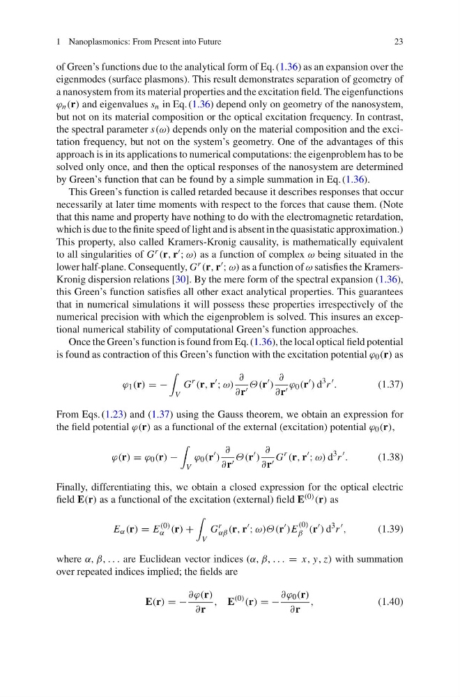
Once the Green’s function is found from Eq. (1.36), the local optical field potential
is found as contraction of this Green’s function with the excitation potential ϕ 0 (r) as
ϕ 1 (r) = −
V
G
r
(r, r
; ω)
∂
∂r Θ(r
)
∂
∂r ϕ 0 (r
) d
3 r
.
(1.37)
From Eqs. (1.23) and (1.37) using the Gauss theorem, we obtain an expression for
the field potential ϕ(r) as a functional of the external (excitation) potential ϕ 0 (r),
ϕ(r) = ϕ 0 (r) −
V
ϕ 0 (r
)
∂
∂r Θ(r
)
∂
∂r G
r
(r, r
; ω) d
3 r
.
(1.38)
Finally, differentiating this, we obtain a closed expression for the optical electric
field E(r) as a functional of the excitation (external) field E (0) (r) as
E α (r) = E
(0)
α (r) +
V
G
r
αβ (r, r
; ω)Θ(r
)E
(0)
β (r
) d
3 r
,
(1.39)
where α, β, . . . are Euclidean vector indices (α, β, . . . = x, y, z) with summation
over repeated indices implied; the fields are
E(r) = −
∂ϕ(r)
∂r
, E
(0)
(r) = −
∂ϕ 0 (r)
∂r
,
(1.40)
23
of Green’s functions due to the analytical form of Eq. (1.36) as an expansion over the
eigenmodes (surface plasmons). This result demonstrates separation of geometry of
a nanosystem from its material properties and the excitation field. The eigenfunctions
ϕ n (r) and eigenvalues s n in Eq. (1.36) depend only on geometry of the nanosystem,
but not on its material composition or the optical excitation frequency. In contrast,
the spectral parameter s(ω) depends only on the material composition and the excitation frequency, but not on the system’s geometry. One of the advantages of this
approach is in its applications to numerical computations: the eigenproblem has to be
solved only once, and then the optical responses of the nanosystem are determined
by Green’s function that can be found by a simple summation in Eq. (1.36).
This Green’s function is called retarded because it describes responses that occur
necessarily at later time moments with respect to the forces that cause them. (Note
that this name and property have nothing to do with the electromagnetic retardation,
which is due to the finite speed of light and is absent in the quasistatic approximation.)
This property, also called Kramers-Kronig causality, is mathematically equivalent
to all singularities of G r (r, r ; ω) as a function of complex ω being situated in the
lower half-plane. Consequently, G r (r, r ; ω) as a function of ω satisfies the KramersKronig dispersion relations [30]. By the mere form of the spectral expansion (1.36),
this Green’s function satisfies all other exact analytical properties. This guarantees
that in numerical simulations it will possess these properties irrespectively of the
numerical precision with which the eigenproblem is solved. This insures an exceptional numerical stability of computational Green’s function approaches.
Once the Green’s function is found from Eq. (1.36), the local optical field potential
is found as contraction of this Green’s function with the excitation potential ϕ 0 (r) as
ϕ 1 (r) = −
V
G
r
(r, r
; ω)
∂
∂r Θ(r
)
∂
∂r ϕ 0 (r
) d
3 r
.
(1.37)
From Eqs. (1.23) and (1.37) using the Gauss theorem, we obtain an expression for
the field potential ϕ(r) as a functional of the external (excitation) potential ϕ 0 (r),
ϕ(r) = ϕ 0 (r) −
V
ϕ 0 (r
)
∂
∂r Θ(r
)
∂
∂r G
r
(r, r
; ω) d
3 r
.
(1.38)
Finally, differentiating this, we obtain a closed expression for the optical electric
field E(r) as a functional of the excitation (external) field E (0) (r) as
E α (r) = E
(0)
α (r) +
V
G
r
αβ (r, r
; ω)Θ(r
)E
(0)
β (r
) d
3 r
,
(1.39)
where α, β, . . . are Euclidean vector indices (α, β, . . . = x, y, z) with summation
over repeated indices implied; the fields are
E(r) = −
∂ϕ(r)
∂r
, E
(0)
(r) = −
∂ϕ 0 (r)
∂r
,
(1.40)