

3 Theoretical Models of Light Scattering and Absorption
49
T =
I
I 0
= ex p(−μ a t)
(3.11)
Equation 3.11 is compatible with the Bouguer (3.1) and Beer (3.3) equations that
opened this chapter, though the absorption coefficient μ a is framed differently than
either the ε in Eq. 3.1 or the κ in Eq. 3.3. Beer’s Law, for example, commonly uses
base 10 logarithms (as in Eq. 3.3) rather than natural logarithms. Beer’s Law also
separates the concentration and the molar absorptivity into two separate parameters,
while the μ a in Eq. 3.11 is a holistic coefficient that is effected by both of these
factors.
In the absence of scatter, light only moves in one direction. It is attenuated by
absorption, so the intensity of the light (T) is a function of position (d) as quantified
in Eq. 3.11, but only one “flux” is needed to describe the process: at any given point,
all of the light that has not been absorbed is moving forward along its original path.
By contrast, in a scattering sample, light can be moving in literally any direction
when it enters or exits a layer.
In a “two-flux” model of a scattering sample, we simply consider the light that
enters and exits a particular layer as moving “forward” or “backward.” If light strikes
the front surface of a layer and exits the back surface, then we say it has been
transmitted through the layer and moves “forward” into the next layer. The model does
not distinguish between the various angles and paths the light could have followed
through the layer. Similarly, if light strikes the front surface of a layer, reverses
direction, and is re-emitted from the front surface, it contributes to the “backward”
flux that enters the rear surface of the previous layer.
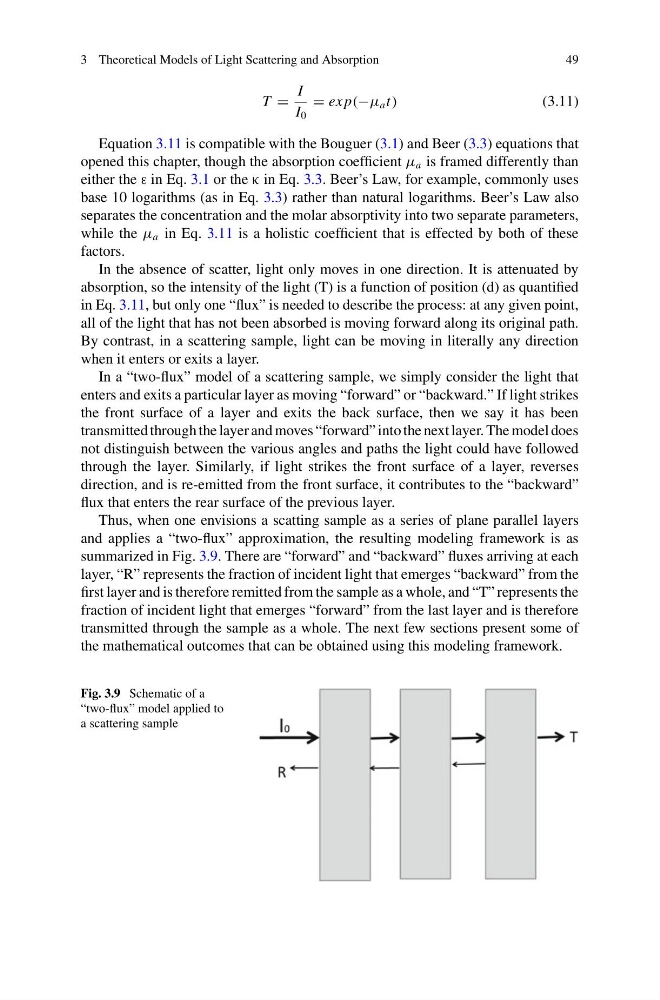
Thus, when one envisions a scatting sample as a series of plane parallel layers
and applies a “two-flux” approximation, the resulting modeling framework is as
summarized in Fig. 3.9. There are “forward” and “backward” fluxes arriving at each
layer, “R” represents the fraction of incident light that emerges “backward” from the
first layer and is therefore remitted from the sample as a whole, and “T” represents the
fraction of incident light that emerges “forward” from the last layer and is therefore
transmitted through the sample as a whole. The next few sections present some of
the mathematical outcomes that can be obtained using this modeling framework.
Fig. 3.9 Schematic of a
“two-flux” model applied to
a scattering sample
49
T =
I
I 0
= ex p(−μ a t)
(3.11)
Equation 3.11 is compatible with the Bouguer (3.1) and Beer (3.3) equations that
opened this chapter, though the absorption coefficient μ a is framed differently than
either the ε in Eq. 3.1 or the κ in Eq. 3.3. Beer’s Law, for example, commonly uses
base 10 logarithms (as in Eq. 3.3) rather than natural logarithms. Beer’s Law also
separates the concentration and the molar absorptivity into two separate parameters,
while the μ a in Eq. 3.11 is a holistic coefficient that is effected by both of these
factors.
In the absence of scatter, light only moves in one direction. It is attenuated by
absorption, so the intensity of the light (T) is a function of position (d) as quantified
in Eq. 3.11, but only one “flux” is needed to describe the process: at any given point,
all of the light that has not been absorbed is moving forward along its original path.
By contrast, in a scattering sample, light can be moving in literally any direction
when it enters or exits a layer.
In a “two-flux” model of a scattering sample, we simply consider the light that
enters and exits a particular layer as moving “forward” or “backward.” If light strikes
the front surface of a layer and exits the back surface, then we say it has been
transmitted through the layer and moves “forward” into the next layer. The model does
not distinguish between the various angles and paths the light could have followed
through the layer. Similarly, if light strikes the front surface of a layer, reverses
direction, and is re-emitted from the front surface, it contributes to the “backward”
flux that enters the rear surface of the previous layer.
Thus, when one envisions a scatting sample as a series of plane parallel layers
and applies a “two-flux” approximation, the resulting modeling framework is as
summarized in Fig. 3.9. There are “forward” and “backward” fluxes arriving at each
layer, “R” represents the fraction of incident light that emerges “backward” from the
first layer and is therefore remitted from the sample as a whole, and “T” represents the
fraction of incident light that emerges “forward” from the last layer and is therefore
transmitted through the sample as a whole. The next few sections present some of
the mathematical outcomes that can be obtained using this modeling framework.
Fig. 3.9 Schematic of a
“two-flux” model applied to
a scattering sample