

170
K. M. Sørensen et al.
8
1 0
1 2
1 4
1 6
1 8
2 0
2 2
Protein measured [%]
8
10
12
14
16
18
20
22
Protein CV predicted [%]
Variety 1
Variety 2
Variety 3
Variety 4
Variety 5
3 components
R2 = 0.94
RMSECV = 0.75
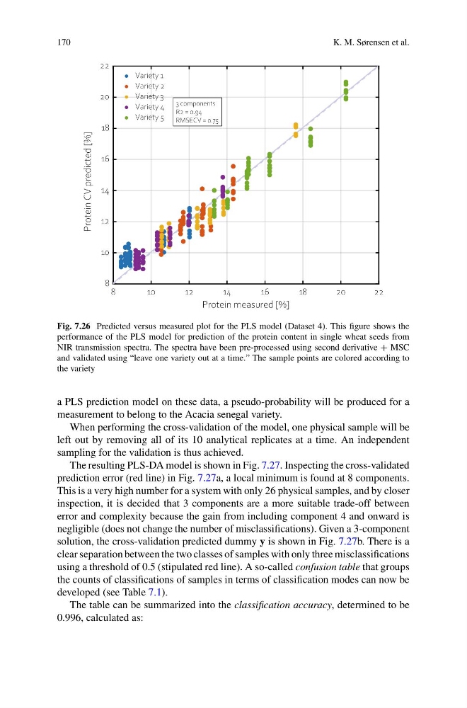
Fig. 7.26 Predicted versus measured plot for the PLS model (Dataset 4). This figure shows the
performance of the PLS model for prediction of the protein content in single wheat seeds from
NIR transmission spectra. The spectra have been pre-processed using second derivative + MSC
and validated using “leave one variety out at a time.” The sample points are colored according to
the variety
a PLS prediction model on these data, a pseudo-probability will be produced for a
measurement to belong to the Acacia senegal variety.
When performing the cross-validation of the model, one physical sample will be
left out by removing all of its 10 analytical replicates at a time. An independent
sampling for the validation is thus achieved.
The resulting PLS-DA model is shown in Fig. 7.27. Inspecting the cross-validated
prediction error (red line) in Fig. 7.27a, a local minimum is found at 8 components.
This is a very high number for a system with only 26 physical samples, and by closer
inspection, it is decided that 3 components are a more suitable trade-off between
error and complexity because the gain from including component 4 and onward is
negligible (does not change the number of misclassifications). Given a 3-component
solution, the cross-validation predicted dummy y is shown in Fig. 7.27b. There is a
clear separation between the two classes of samples with only three misclassifications
using a threshold of 0.5 (stipulated red line). A so-called confusion table that groups
the counts of classifications of samples in terms of classification modes can now be
developed (see Table 7.1).
The table can be summarized into the classification accuracy, determined to be
0.996, calculated as:
K. M. Sørensen et al.
8
1 0
1 2
1 4
1 6
1 8
2 0
2 2
Protein measured [%]
8
10
12
14
16
18
20
22
Protein CV predicted [%]
Variety 1
Variety 2
Variety 3
Variety 4
Variety 5
3 components
R2 = 0.94
RMSECV = 0.75
Fig. 7.26 Predicted versus measured plot for the PLS model (Dataset 4). This figure shows the
performance of the PLS model for prediction of the protein content in single wheat seeds from
NIR transmission spectra. The spectra have been pre-processed using second derivative + MSC
and validated using “leave one variety out at a time.” The sample points are colored according to
the variety
a PLS prediction model on these data, a pseudo-probability will be produced for a
measurement to belong to the Acacia senegal variety.
When performing the cross-validation of the model, one physical sample will be
left out by removing all of its 10 analytical replicates at a time. An independent
sampling for the validation is thus achieved.
The resulting PLS-DA model is shown in Fig. 7.27. Inspecting the cross-validated
prediction error (red line) in Fig. 7.27a, a local minimum is found at 8 components.
This is a very high number for a system with only 26 physical samples, and by closer
inspection, it is decided that 3 components are a more suitable trade-off between
error and complexity because the gain from including component 4 and onward is
negligible (does not change the number of misclassifications). Given a 3-component
solution, the cross-validation predicted dummy y is shown in Fig. 7.27b. There is a
clear separation between the two classes of samples with only three misclassifications
using a threshold of 0.5 (stipulated red line). A so-called confusion table that groups
the counts of classifications of samples in terms of classification modes can now be
developed (see Table 7.1).
The table can be summarized into the classification accuracy, determined to be
0.996, calculated as: