

140
K. M. Sørensen et al.
7.2.2 Spectral (Second) Derivatives
The classical method to eliminate spectral offsets (additive effects) and slopes (multiplicative effects) is to calculate derivatives. The first-order derivative is calculated as
the difference between two subsequent spectral variables; the second-order derivative is then calculated by calculating the difference between two successive points
of the first-order derivative spectra:
x
m = x m − x m−1
x
m = x
m − x
m−1 = x m − 2x m + x m−2
(7.10)
The second derivate of a spectrum will have two implications: (a) The additive
effect will be eliminated by the first derivative, and (b) the multiplicative effect will
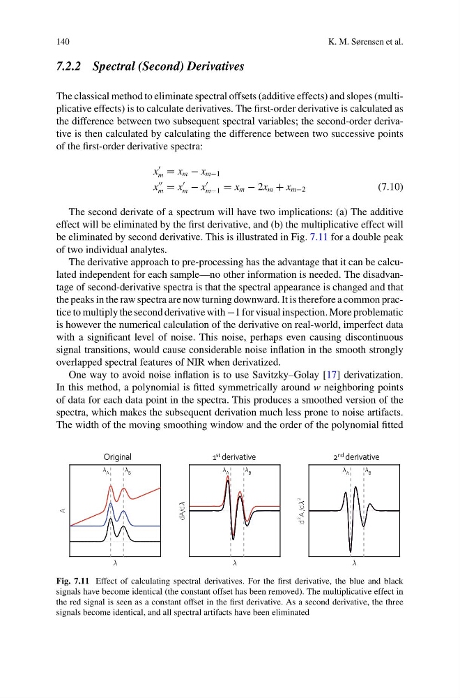
be eliminated by second derivative. This is illustrated in Fig. 7.11 for a double peak
of two individual analytes.
The derivative approach to pre-processing has the advantage that it can be calculated independent for each sample—no other information is needed. The disadvantage of second-derivative spectra is that the spectral appearance is changed and that
the peaks in the raw spectra are now turning downward. It is therefore a common practice to multiply the second derivative with −1 for visual inspection. More problematic
is however the numerical calculation of the derivative on real-world, imperfect data
with a significant level of noise. This noise, perhaps even causing discontinuous
signal transitions, would cause considerable noise inflation in the smooth strongly
overlapped spectral features of NIR when derivatized.
One way to avoid noise inflation is to use Savitzky–Golay [17] derivatization.
In this method, a polynomial is fitted symmetrically around w neighboring points
of data for each data point in the spectra. This produces a smoothed version of the
spectra, which makes the subsequent derivation much less prone to noise artifacts.
The width of the moving smoothing window and the order of the polynomial fitted
A
A
B
A
B
dA/d
A
B
A
B
d
2
A /d
2
A
B
A
B
2 nd derivative
Original
1 st derivative
Fig. 7.11 Effect of calculating spectral derivatives. For the first derivative, the blue and black
signals have become identical (the constant offset has been removed). The multiplicative effect in
the red signal is seen as a constant offset in the first derivative. As a second derivative, the three
signals become identical, and all spectral artifacts have been eliminated
K. M. Sørensen et al.
7.2.2 Spectral (Second) Derivatives
The classical method to eliminate spectral offsets (additive effects) and slopes (multiplicative effects) is to calculate derivatives. The first-order derivative is calculated as
the difference between two subsequent spectral variables; the second-order derivative is then calculated by calculating the difference between two successive points
of the first-order derivative spectra:
x
m = x m − x m−1
x
m = x
m − x
m−1 = x m − 2x m + x m−2
(7.10)
The second derivate of a spectrum will have two implications: (a) The additive
effect will be eliminated by the first derivative, and (b) the multiplicative effect will
be eliminated by second derivative. This is illustrated in Fig. 7.11 for a double peak
of two individual analytes.
The derivative approach to pre-processing has the advantage that it can be calculated independent for each sample—no other information is needed. The disadvantage of second-derivative spectra is that the spectral appearance is changed and that
the peaks in the raw spectra are now turning downward. It is therefore a common practice to multiply the second derivative with −1 for visual inspection. More problematic
is however the numerical calculation of the derivative on real-world, imperfect data
with a significant level of noise. This noise, perhaps even causing discontinuous
signal transitions, would cause considerable noise inflation in the smooth strongly
overlapped spectral features of NIR when derivatized.
One way to avoid noise inflation is to use Savitzky–Golay [17] derivatization.
In this method, a polynomial is fitted symmetrically around w neighboring points
of data for each data point in the spectra. This produces a smoothed version of the
spectra, which makes the subsequent derivation much less prone to noise artifacts.
The width of the moving smoothing window and the order of the polynomial fitted
A
A
B
A
B
dA/d
A
B
A
B
d
2
A /d
2
A
B
A
B
2 nd derivative
Original
1 st derivative
Fig. 7.11 Effect of calculating spectral derivatives. For the first derivative, the blue and black
signals have become identical (the constant offset has been removed). The multiplicative effect in
the red signal is seen as a constant offset in the first derivative. As a second derivative, the three
signals become identical, and all spectral artifacts have been eliminated