

7 NIR Data Exploration and Regression by Chemometrics—A Primer
139
0
0.1
0.2
0.3
0.4
0.5
0.6
0.7
0.8
Reference spectrum
X ref
0
0.1
0.2
0.3
0.4
0.5
0.6
0.7
0.8
Spectrum to be corrected
X
corr
Δx
Δy
Δy
Δx
b 1 =
b 0
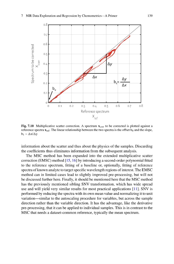
Fig. 7.10 Multiplicative scatter correction. A spectrum x corr to be corrected is plotted against a
reference spectra x ref . The linear relationship between the two spectra is the offset b 0 and the slope,
b 1 ~ x/
information about the scatter and thus about the physics of the samples. Discarding
the coefficients thus eliminates information from the subsequent analysis.
The MSC method has been expanded into the extended multiplicative scatter
correction (EMSC) method [15, 16] by introducing a second-order polynomial fitted
to the reference spectrum, fitting of a baseline or, optionally, fitting of reference
spectra of known analyte to target specific wavelength regions of interest. The EMSC
method can in limited cases lead to slightly improved pre-processing, but will not
be discussed further here. Finally, it should be mentioned here that the MSC method
has the previously mentioned sibling SNV transformation, which has wide spread
use and will yield very similar results for most practical applications [11]. SNV is
performed by reducing the spectra with its own mean value and normalizing it to unit
variation—similar to the autoscaling procedure for variables, but across the sample
direction rather than the variable direction. It has the advantage, like the derivative
pre-processing, that it can be applied to individual samples. This is in contrast to the
MSC that needs a dataset-common reference, typically the mean spectrum.
139
0
0.1
0.2
0.3
0.4
0.5
0.6
0.7
0.8
Reference spectrum
X ref
0
0.1
0.2
0.3
0.4
0.5
0.6
0.7
0.8
Spectrum to be corrected
X
corr
Δx
Δy
Δy
Δx
b 1 =
b 0
Fig. 7.10 Multiplicative scatter correction. A spectrum x corr to be corrected is plotted against a
reference spectra x ref . The linear relationship between the two spectra is the offset b 0 and the slope,
b 1 ~ x/
information about the scatter and thus about the physics of the samples. Discarding
the coefficients thus eliminates information from the subsequent analysis.
The MSC method has been expanded into the extended multiplicative scatter
correction (EMSC) method [15, 16] by introducing a second-order polynomial fitted
to the reference spectrum, fitting of a baseline or, optionally, fitting of reference
spectra of known analyte to target specific wavelength regions of interest. The EMSC
method can in limited cases lead to slightly improved pre-processing, but will not
be discussed further here. Finally, it should be mentioned here that the MSC method
has the previously mentioned sibling SNV transformation, which has wide spread
use and will yield very similar results for most practical applications [11]. SNV is
performed by reducing the spectra with its own mean value and normalizing it to unit
variation—similar to the autoscaling procedure for variables, but across the sample
direction rather than the variable direction. It has the advantage, like the derivative
pre-processing, that it can be applied to individual samples. This is in contrast to the
MSC that needs a dataset-common reference, typically the mean spectrum.