

178
S. Cerveny and J. Swenson
4 The Dynamics of Water in Amorphous Water Solutions
at Low Temperatures by BDS
In this section, we review the dynamics of the aqueous solutions showed in Fig. 2
as seen by broadband dielectric spectroscopy when water remains amorphous for
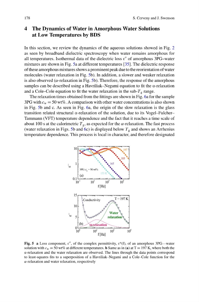
all temperatures. Isothermal data of the dielectric loss ε
of amorphous 3PG–water
mixtures are shown in Fig. 5a at different temperatures [35]. The dielectric response
of these amorphous mixtures shows a prominent peak due to the reorientation of water
molecules (water relaxation in Fig. 5b). In addition, a slower and weaker relaxation
is also observed (α-relaxation in Fig. 5b). Therefore, the response of the amorphous
samples can be described using a Havriliak–Negami equation to fit the α-relaxation
and a Cole–Cole equation to fit the water relaxation in the sub-T g range.
The relaxation times obtained from the fittings are shown in Fig. 6a for the sample
3PG with c w = 50 wt%. A comparison with other water concentrations is also shown
in Fig. 5b and c. As seen in Fig. 6a, the origin of the slow relaxation is the glass
transition related structural α-relaxation of the solution, due to its Vogel–Fulcher–
Tammann (VFT) temperature dependence and the fact that it reaches a time scale of
about 100 s at the calorimetric T g , as expected for the α-relaxation. The fast process
(water relaxation in Figs. 5b and 6c) is displayed below T g and shows an Arrhenius
temperature dependence. This process is local in character, and therefore designated
10
-1
10
1
10
3
10
5
0.1
1
10
3PG: c w = 50 wt%
(a)
155 K
197
185
165
ε´´
f [Hz]
10
0
10
2
10
4
10
6
0
5
10
15
(b)
Conductivity
T = 197 K
Water
relaxation
α-relaxation
ε´´
f [Hz]
Fig. 5 a Loss component, ε , of the complex permittivity, ε*(f), of an amorphous 3PG—water
solution with c w = 50 wt% at different temperatures. b Same as in (a) at T = 197 K, where both the
α-relaxation and the water relaxation are observed. The lines through the data points correspond
to least-squares fits to a superposition of a Havriliak–Negami and a Cole–Cole function for the
α-relaxation and water relaxation, respectively
S. Cerveny and J. Swenson
4 The Dynamics of Water in Amorphous Water Solutions
at Low Temperatures by BDS
In this section, we review the dynamics of the aqueous solutions showed in Fig. 2
as seen by broadband dielectric spectroscopy when water remains amorphous for
all temperatures. Isothermal data of the dielectric loss ε
of amorphous 3PG–water
mixtures are shown in Fig. 5a at different temperatures [35]. The dielectric response
of these amorphous mixtures shows a prominent peak due to the reorientation of water
molecules (water relaxation in Fig. 5b). In addition, a slower and weaker relaxation
is also observed (α-relaxation in Fig. 5b). Therefore, the response of the amorphous
samples can be described using a Havriliak–Negami equation to fit the α-relaxation
and a Cole–Cole equation to fit the water relaxation in the sub-T g range.
The relaxation times obtained from the fittings are shown in Fig. 6a for the sample
3PG with c w = 50 wt%. A comparison with other water concentrations is also shown
in Fig. 5b and c. As seen in Fig. 6a, the origin of the slow relaxation is the glass
transition related structural α-relaxation of the solution, due to its Vogel–Fulcher–
Tammann (VFT) temperature dependence and the fact that it reaches a time scale of
about 100 s at the calorimetric T g , as expected for the α-relaxation. The fast process
(water relaxation in Figs. 5b and 6c) is displayed below T g and shows an Arrhenius
temperature dependence. This process is local in character, and therefore designated
10
-1
10
1
10
3
10
5
0.1
1
10
3PG: c w = 50 wt%
(a)
155 K
197
185
165
ε´´
f [Hz]
10
0
10
2
10
4
10
6
0
5
10
15
(b)
Conductivity
T = 197 K
Water
relaxation
α-relaxation
ε´´
f [Hz]
Fig. 5 a Loss component, ε , of the complex permittivity, ε*(f), of an amorphous 3PG—water
solution with c w = 50 wt% at different temperatures. b Same as in (a) at T = 197 K, where both the
α-relaxation and the water relaxation are observed. The lines through the data points correspond
to least-squares fits to a superposition of a Havriliak–Negami and a Cole–Cole function for the
α-relaxation and water relaxation, respectively