

56
K. P. Satheesh
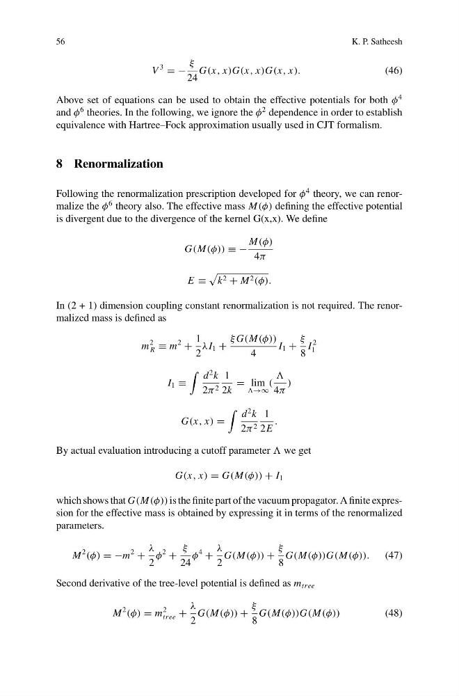
V
3
= −
ξ
24
G(x, x)G(x, x)G(x, x).
(46)
Above set of equations can be used to obtain the effective potentials for both φ
4
and φ
6 theories. In the following, we ignore the φ
2 dependence in order to establish
equivalence with Hartree–Fock approximation usually used in CJT formalism.
8 Renormalization
Following the renormalization prescription developed for φ
4 theory, we can renormalize the φ
6 theory also. The effective mass M(φ) defining the effective potential
is divergent due to the divergence of the kernel G(x,x). We define
G(M(φ)) ≡ −
M(φ)
4π
E ≡
k 2 + M 2 (φ).
In (2 + 1) dimension coupling constant renormalization is not required. The renormalized mass is defined as
m
2
R ≡ m
2
+
1
2
λI 1 +
ξ G(M(φ))
4
I 1 +
ξ
8
I
2
1
I 1 ≡
d
2 k
2π 2
1
2k
= lim
→∞
(
4π
)
G(x, x) =
d
2 k
2π 2
1
2E
.
By actual evaluation introducing a cutoff parameter we get
G(x, x) = G(M(φ)) + I 1
which shows that G(M(φ)) is the finite part of the vacuum propagator. A finite expression for the effective mass is obtained by expressing it in terms of the renormalized
parameters.
M
2
(φ) = −m
2
+
λ
2
φ
2
+
ξ
24
φ
4
+
λ
2
G(M(φ)) +
ξ
8
G(M(φ))G(M(φ)).
(47)
Second derivative of the tree-level potential is defined as m tree
M
2
(φ) = m
2
tree +
λ
2
G(M(φ)) +
ξ
8
G(M(φ))G(M(φ))
(48)
K. P. Satheesh
V
3
= −
ξ
24
G(x, x)G(x, x)G(x, x).
(46)
Above set of equations can be used to obtain the effective potentials for both φ
4
and φ
6 theories. In the following, we ignore the φ
2 dependence in order to establish
equivalence with Hartree–Fock approximation usually used in CJT formalism.
8 Renormalization
Following the renormalization prescription developed for φ
4 theory, we can renormalize the φ
6 theory also. The effective mass M(φ) defining the effective potential
is divergent due to the divergence of the kernel G(x,x). We define
G(M(φ)) ≡ −
M(φ)
4π
E ≡
k 2 + M 2 (φ).
In (2 + 1) dimension coupling constant renormalization is not required. The renormalized mass is defined as
m
2
R ≡ m
2
+
1
2
λI 1 +
ξ G(M(φ))
4
I 1 +
ξ
8
I
2
1
I 1 ≡
d
2 k
2π 2
1
2k
= lim
→∞
(
4π
)
G(x, x) =
d
2 k
2π 2
1
2E
.
By actual evaluation introducing a cutoff parameter we get
G(x, x) = G(M(φ)) + I 1
which shows that G(M(φ)) is the finite part of the vacuum propagator. A finite expression for the effective mass is obtained by expressing it in terms of the renormalized
parameters.
M
2
(φ) = −m
2
+
λ
2
φ
2
+
ξ
24
φ
4
+
λ
2
G(M(φ)) +
ξ
8
G(M(φ))G(M(φ)).
(47)
Second derivative of the tree-level potential is defined as m tree
M
2
(φ) = m
2
tree +
λ
2
G(M(φ)) +
ξ
8
G(M(φ))G(M(φ))
(48)