

Aspects of Schrödinger Picture Formalism
55
∂ V
∂φ
= φ
m
2
+
λ
6
φ
2
+
ξ
120
φ
4
+
λ
2
G(x, x) +
ξ
12
φ
2 G(x, x)
+
ξ
4
φ
2 G(x, x)
= 0
(37)
∂ V
∂ M 2 = −
1
2
M − m
2
−
λ
2
φ
2
−
ξ
24
φ
4
−
λ
4
φ
2 G(x, x)
−
ξ
8
G(x, x)G(x, x)
∂G(x, x)
∂ M 2 = 0.
(38)
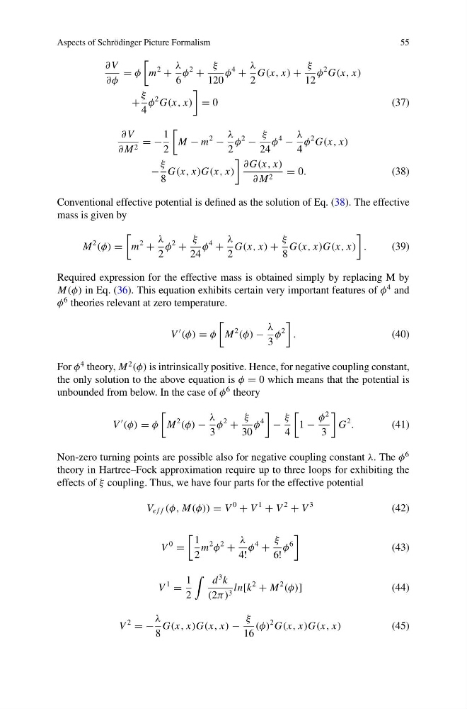
Conventional effective potential is defined as the solution of Eq. (38). The effective
mass is given by
M
2
(φ) =
m
2
+
λ
2
φ
2
+
ξ
24
φ
4
+
λ
2
G(x, x) +
ξ
8
G(x, x)G(x, x)
.
(39)
Required expression for the effective mass is obtained simply by replacing M by
M(φ) in Eq. (36). This equation exhibits certain very important features of φ
4 and
φ
6 theories relevant at zero temperature.
V
(φ) = φ
M
2
(φ) −
λ
3
φ
2
.
(40)
For φ
4 theory, M
2
(φ) is intrinsically positive. Hence, for negative coupling constant,
the only solution to the above equation is φ = 0 which means that the potential is
unbounded from below. In the case of φ
6 theory
V
(φ) = φ
M
2
(φ) −
λ
3
φ
2
+
ξ
30
φ
4
−
ξ
4
1 −
φ
2
3
G
2
.
(41)
Non-zero turning points are possible also for negative coupling constant λ. The φ
6
theory in Hartree–Fock approximation require up to three loops for exhibiting the
effects of ξ coupling. Thus, we have four parts for the effective potential
V e f f (φ, M(φ)) = V
0
+ V
1
+ V
2
+ V
3
(42)
V
0
=
1
2
m
2
φ
2
+
λ
4!
φ
4
+
ξ
6!
φ
6
(43)
V
1
=
1
2
d
3 k
(2π) 3 ln[k
2
+ M
2
(φ)]
(44)
V
2
= −
λ
8
G(x, x)G(x, x) −
ξ
16
(φ)
2 G(x, x)G(x, x)
(45)
55
∂ V
∂φ
= φ
m
2
+
λ
6
φ
2
+
ξ
120
φ
4
+
λ
2
G(x, x) +
ξ
12
φ
2 G(x, x)
+
ξ
4
φ
2 G(x, x)
= 0
(37)
∂ V
∂ M 2 = −
1
2
M − m
2
−
λ
2
φ
2
−
ξ
24
φ
4
−
λ
4
φ
2 G(x, x)
−
ξ
8
G(x, x)G(x, x)
∂G(x, x)
∂ M 2 = 0.
(38)
Conventional effective potential is defined as the solution of Eq. (38). The effective
mass is given by
M
2
(φ) =
m
2
+
λ
2
φ
2
+
ξ
24
φ
4
+
λ
2
G(x, x) +
ξ
8
G(x, x)G(x, x)
.
(39)
Required expression for the effective mass is obtained simply by replacing M by
M(φ) in Eq. (36). This equation exhibits certain very important features of φ
4 and
φ
6 theories relevant at zero temperature.
V
(φ) = φ
M
2
(φ) −
λ
3
φ
2
.
(40)
For φ
4 theory, M
2
(φ) is intrinsically positive. Hence, for negative coupling constant,
the only solution to the above equation is φ = 0 which means that the potential is
unbounded from below. In the case of φ
6 theory
V
(φ) = φ
M
2
(φ) −
λ
3
φ
2
+
ξ
30
φ
4
−
ξ
4
1 −
φ
2
3
G
2
.
(41)
Non-zero turning points are possible also for negative coupling constant λ. The φ
6
theory in Hartree–Fock approximation require up to three loops for exhibiting the
effects of ξ coupling. Thus, we have four parts for the effective potential
V e f f (φ, M(φ)) = V
0
+ V
1
+ V
2
+ V
3
(42)
V
0
=
1
2
m
2
φ
2
+
λ
4!
φ
4
+
ξ
6!
φ
6
(43)
V
1
=
1
2
d
3 k
(2π) 3 ln[k
2
+ M
2
(φ)]
(44)
V
2
= −
λ
8
G(x, x)G(x, x) −
ξ
16
(φ)
2 G(x, x)G(x, x)
(45)