

54
K. P. Satheesh
G(x, x) =
d
ν
2π ν
1
2
k
2
+ m
2
+
λ
2
ˆ
φ
2
+
ξ
24
ˆ
φ
4
×
λ
2
G(x, x) +
ξ
4
ˆ
φ
2 G(x, x) +
ξ
48
G(x, x)
−
1
2
(35)
G(x, x) =
d
ν k
2π ν
1
2(k 2 + M 2 )
1
2
.
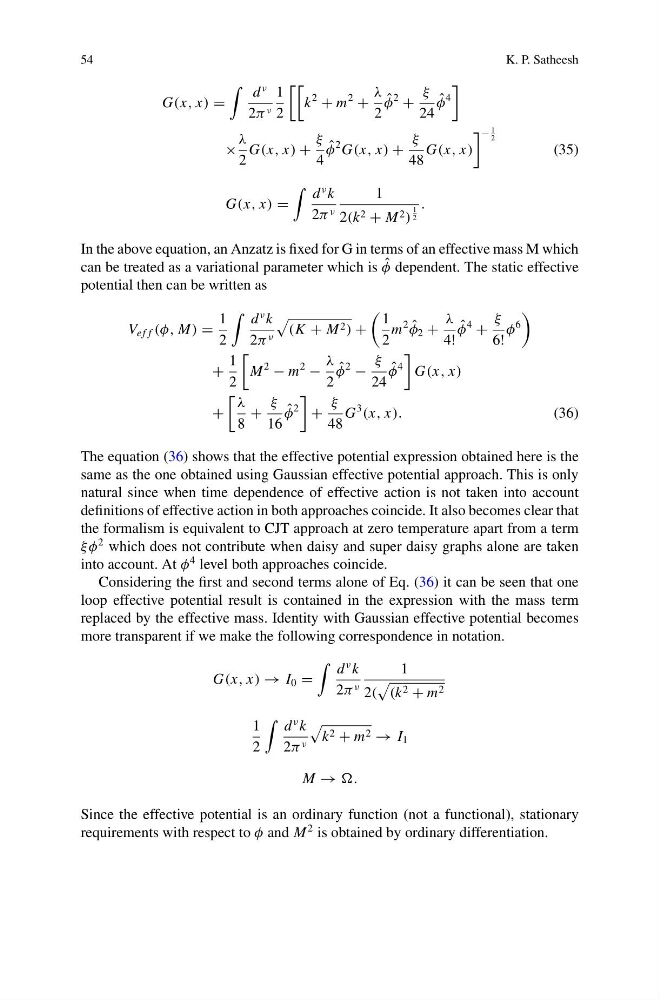
In the above equation, an Anzatz is fixed for G in terms of an effective mass M which
can be treated as a variational parameter which is ˆ
φ dependent. The static effective
potential then can be written as
V e f f (φ, M) =
1
2
d
ν k
2π ν
(K + M 2 ) +
1
2
m
2 ˆ
φ 2 +
λ
4!
ˆ
φ
4
+
ξ
6!
φ
6
+
1
2
M
2
− m
2
−
λ
2
ˆ
φ
2
−
ξ
24
ˆ
φ
4
G(x, x)
+
λ
8
+
ξ
16
ˆ
φ
2
+
ξ
48
G
3
(x, x).
(36)
The equation (36) shows that the effective potential expression obtained here is the
same as the one obtained using Gaussian effective potential approach. This is only
natural since when time dependence of effective action is not taken into account
definitions of effective action in both approaches coincide. It also becomes clear that
the formalism is equivalent to CJT approach at zero temperature apart from a term
ξφ
2 which does not contribute when daisy and super daisy graphs alone are taken
into account. At φ
4 level both approaches coincide.
Considering the first and second terms alone of Eq. (36) it can be seen that one
loop effective potential result is contained in the expression with the mass term
replaced by the effective mass. Identity with Gaussian effective potential becomes
more transparent if we make the following correspondence in notation.
G(x, x) → I 0 =
d
ν k
2π ν
1
2(
(k 2 + m 2
1
2
d
ν k
2π ν
k 2 + m 2 → I 1
M → .
Since the effective potential is an ordinary function (not a functional), stationary
requirements with respect to φ and M
2 is obtained by ordinary differentiation.
K. P. Satheesh
G(x, x) =
d
ν
2π ν
1
2
k
2
+ m
2
+
λ
2
ˆ
φ
2
+
ξ
24
ˆ
φ
4
×
λ
2
G(x, x) +
ξ
4
ˆ
φ
2 G(x, x) +
ξ
48
G(x, x)
−
1
2
(35)
G(x, x) =
d
ν k
2π ν
1
2(k 2 + M 2 )
1
2
.
In the above equation, an Anzatz is fixed for G in terms of an effective mass M which
can be treated as a variational parameter which is ˆ
φ dependent. The static effective
potential then can be written as
V e f f (φ, M) =
1
2
d
ν k
2π ν
(K + M 2 ) +
1
2
m
2 ˆ
φ 2 +
λ
4!
ˆ
φ
4
+
ξ
6!
φ
6
+
1
2
M
2
− m
2
−
λ
2
ˆ
φ
2
−
ξ
24
ˆ
φ
4
G(x, x)
+
λ
8
+
ξ
16
ˆ
φ
2
+
ξ
48
G
3
(x, x).
(36)
The equation (36) shows that the effective potential expression obtained here is the
same as the one obtained using Gaussian effective potential approach. This is only
natural since when time dependence of effective action is not taken into account
definitions of effective action in both approaches coincide. It also becomes clear that
the formalism is equivalent to CJT approach at zero temperature apart from a term
ξφ
2 which does not contribute when daisy and super daisy graphs alone are taken
into account. At φ
4 level both approaches coincide.
Considering the first and second terms alone of Eq. (36) it can be seen that one
loop effective potential result is contained in the expression with the mass term
replaced by the effective mass. Identity with Gaussian effective potential becomes
more transparent if we make the following correspondence in notation.
G(x, x) → I 0 =
d
ν k
2π ν
1
2(
(k 2 + m 2
1
2
d
ν k
2π ν
k 2 + m 2 → I 1
M → .
Since the effective potential is an ordinary function (not a functional), stationary
requirements with respect to φ and M
2 is obtained by ordinary differentiation.