

Aspects of Schrödinger Picture Formalism
53
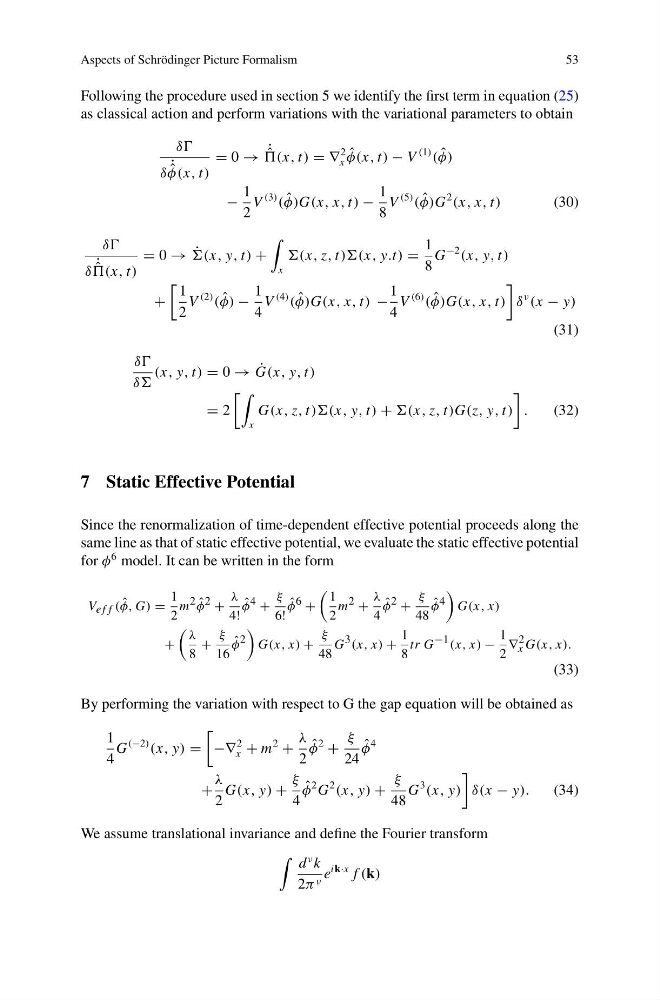
Following the procedure used in section 5 we identify the first term in equation (25)
as classical action and perform variations with the variational parameters to obtain
δδ
δ ˙ ˆ
φ(x, t)
= 0 → ˙ ˆ
(x, t) = ∇
2
x
ˆ
φ(x, t) − V
(1)
( ˆ
φ)
−
1
2
V
(3)
( ˆ
φ)G(x, x, t) −
1
8
V
(5)
( ˆ
φ)G
2
(x, x, t)
(30)
δδ
δ ˙ ˆ
(x, t)
= 0 → ˙
(x, y, t) +
x
(x, z, t))(x, y.t) =
1
8
G
−2
(x, y, t)
+
1
2
V
(2)
( ˆ
φ) −
1
4
V
(4)
( ˆ
φ)G(x, x, t) −
1
4
V
(6)
( ˆ
φ)G(x, x, t)
δ
ν
(x − y)
(31)
δδ
δδ
(x, y, t) = 0 → ˙
G(x, y, t)
= 2
x
G(x, z, t))(x, y, t) + (x, z, t)G(z, y, t)
.
(32)
7 Static Effective Potential
Since the renormalization of time-dependent effective potential proceeds along the
same line as that of static effective potential, we evaluate the static effective potential
for φ
6 model. It can be written in the form
V e f f ( ˆ
φ, G) =
1
2
m 2 ˆ
φ 2 +
λ
4!
ˆ
φ 4 +
ξ
6!
ˆ
φ 6 +
1
2
m 2 +
λ
4
ˆ
φ 2 +
ξ
48
ˆ
φ 4
G(x, x)
+
λ
8
+
ξ
16
ˆ
φ 2
G(x, x) +
ξ
48
G 3 (x, x) +
1
8
tr G −1 (x, x) −
1
2
∇ 2
x G(x, x).
(33)
By performing the variation with respect to G the gap equation will be obtained as
1
4
G
(−2)
(x, y) =
−∇
2
x + m
2
+
λ
2
ˆ
φ
2
+
ξ
24
ˆ
φ
4
+
λ
2
G(x, y) +
ξ
4
ˆ
φ
2 G
2
(x, y) +
ξ
48
G
3
(x, y)
δ(x − y).
(34)
We assume translational invariance and define the Fourier transform
d
ν k
2π ν e
ik·x f (k)
53
Following the procedure used in section 5 we identify the first term in equation (25)
as classical action and perform variations with the variational parameters to obtain
δδ
δ ˙ ˆ
φ(x, t)
= 0 → ˙ ˆ
(x, t) = ∇
2
x
ˆ
φ(x, t) − V
(1)
( ˆ
φ)
−
1
2
V
(3)
( ˆ
φ)G(x, x, t) −
1
8
V
(5)
( ˆ
φ)G
2
(x, x, t)
(30)
δδ
δ ˙ ˆ
(x, t)
= 0 → ˙
(x, y, t) +
x
(x, z, t))(x, y.t) =
1
8
G
−2
(x, y, t)
+
1
2
V
(2)
( ˆ
φ) −
1
4
V
(4)
( ˆ
φ)G(x, x, t) −
1
4
V
(6)
( ˆ
φ)G(x, x, t)
δ
ν
(x − y)
(31)
δδ
δδ
(x, y, t) = 0 → ˙
G(x, y, t)
= 2
x
G(x, z, t))(x, y, t) + (x, z, t)G(z, y, t)
.
(32)
7 Static Effective Potential
Since the renormalization of time-dependent effective potential proceeds along the
same line as that of static effective potential, we evaluate the static effective potential
for φ
6 model. It can be written in the form
V e f f ( ˆ
φ, G) =
1
2
m 2 ˆ
φ 2 +
λ
4!
ˆ
φ 4 +
ξ
6!
ˆ
φ 6 +
1
2
m 2 +
λ
4
ˆ
φ 2 +
ξ
48
ˆ
φ 4
G(x, x)
+
λ
8
+
ξ
16
ˆ
φ 2
G(x, x) +
ξ
48
G 3 (x, x) +
1
8
tr G −1 (x, x) −
1
2
∇ 2
x G(x, x).
(33)
By performing the variation with respect to G the gap equation will be obtained as
1
4
G
(−2)
(x, y) =
−∇
2
x + m
2
+
λ
2
ˆ
φ
2
+
ξ
24
ˆ
φ
4
+
λ
2
G(x, y) +
ξ
4
ˆ
φ
2 G
2
(x, y) +
ξ
48
G
3
(x, y)
δ(x − y).
(34)
We assume translational invariance and define the Fourier transform
d
ν k
2π ν e
ik·x f (k)