

50
K. P. Satheesh
−i
δ
δφ(x)
= ( ˆ
x, t)
(21)
φ(x)φ(y) = φ( ˆ
x, t) ˆ
y, t) + G(x, y, t)
(22)
i
∂
∂t
=
x
ˆ
(x, t) ˙ ˆ
φ(x, t) +
x,y
(x, y, t) ˙
G(x, y, t)
(23)
V
(n)
(φ) ≡
d
n V (φ)
d ˆ
φ n
.
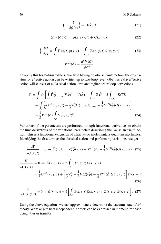
To apply this formalism to the scalar field having quartic self-interaction, the expression for effective action can be written up to two-loop level. Obviously the effective
action will consist of a classical action term and higher order loop corrections.
=
dt
x
ˆ
˙ ˆ
φ −
1
2
(∇ ˆ
φ)
2
− V ( ˆ
φ) +
x,y
˙
G − 2
x,y,z
G
−
x
1
8
G
−1
(x, x, t) −
1
2
∇
2
x G(x, y, t)| x=y +
1
2
V
(2)
( ˆ
φ)G(x, x, t)
−
1
8
V
(4)
( ˆ
φ)
x
G(x, x, t)
2
.
(24)
Variations of the parameters are performed through functional derivatives to obtain
the time derivatives of the variational parameters describing the Gaussian trial function. This is a functional extension of what we do in elementary quantum mechanics.
Identifying the first term as the classical action and performing variations, we get
δδ
δ ˙ ˆ
φ(x, t)
= 0 → ˙ ˆ
(x, t) = ∇
2
x
ˆ
φ(x, t) − V
(1)
( ˆ
φ) −
1
2
V
(3)
( ˆ
φ)G(x, x, t) (25)
δδ
δ ˙ ˆ
(x, t)
= 0 → ˙
(x, y, t) + 2
x
(x, z, t))(x, y, t)
=
1
8
G
−2
(x, y, t) +
1
2
∇
2
x −
1
2
V (2)( ˆ
φ) −
1
4
V
(4)
( ˆ
φ)G(x, x, t)
δ
ν
(x − y)
(26)
δδ
δδ(x, y, t)
= 0 → ˙
G(x, y, t) = 2
x
G(x, z, t))(x, y, t) + (x, z, t)G(z, y, t)
. (27)
Using the above equations we can approximately determine the vacuum state of φ
4
theory. We take ˆ
φ to be x independent. Kernels can be expressed in momentum space
using Fourier transform
K. P. Satheesh
−i
δ
δφ(x)
= ( ˆ
x, t)
(21)
φ(x)φ(y) = φ( ˆ
x, t) ˆ
y, t) + G(x, y, t)
(22)
i
∂
∂t
=
x
ˆ
(x, t) ˙ ˆ
φ(x, t) +
x,y
(x, y, t) ˙
G(x, y, t)
(23)
V
(n)
(φ) ≡
d
n V (φ)
d ˆ
φ n
.
To apply this formalism to the scalar field having quartic self-interaction, the expression for effective action can be written up to two-loop level. Obviously the effective
action will consist of a classical action term and higher order loop corrections.
=
dt
x
ˆ
˙ ˆ
φ −
1
2
(∇ ˆ
φ)
2
− V ( ˆ
φ) +
x,y
˙
G − 2
x,y,z
G
−
x
1
8
G
−1
(x, x, t) −
1
2
∇
2
x G(x, y, t)| x=y +
1
2
V
(2)
( ˆ
φ)G(x, x, t)
−
1
8
V
(4)
( ˆ
φ)
x
G(x, x, t)
2
.
(24)
Variations of the parameters are performed through functional derivatives to obtain
the time derivatives of the variational parameters describing the Gaussian trial function. This is a functional extension of what we do in elementary quantum mechanics.
Identifying the first term as the classical action and performing variations, we get
δδ
δ ˙ ˆ
φ(x, t)
= 0 → ˙ ˆ
(x, t) = ∇
2
x
ˆ
φ(x, t) − V
(1)
( ˆ
φ) −
1
2
V
(3)
( ˆ
φ)G(x, x, t) (25)
δδ
δ ˙ ˆ
(x, t)
= 0 → ˙
(x, y, t) + 2
x
(x, z, t))(x, y, t)
=
1
8
G
−2
(x, y, t) +
1
2
∇
2
x −
1
2
V (2)( ˆ
φ) −
1
4
V
(4)
( ˆ
φ)G(x, x, t)
δ
ν
(x − y)
(26)
δδ
δδ(x, y, t)
= 0 → ˙
G(x, y, t) = 2
x
G(x, z, t))(x, y, t) + (x, z, t)G(z, y, t)
. (27)
Using the above equations we can approximately determine the vacuum state of φ
4
theory. We take ˆ
φ to be x independent. Kernels can be expressed in momentum space
using Fourier transform