

Aspects of Schrödinger Picture Formalism
51
G(x, y) =
d
3 p
(2π) 3 e
ip·(x−y) ˜
G(p).
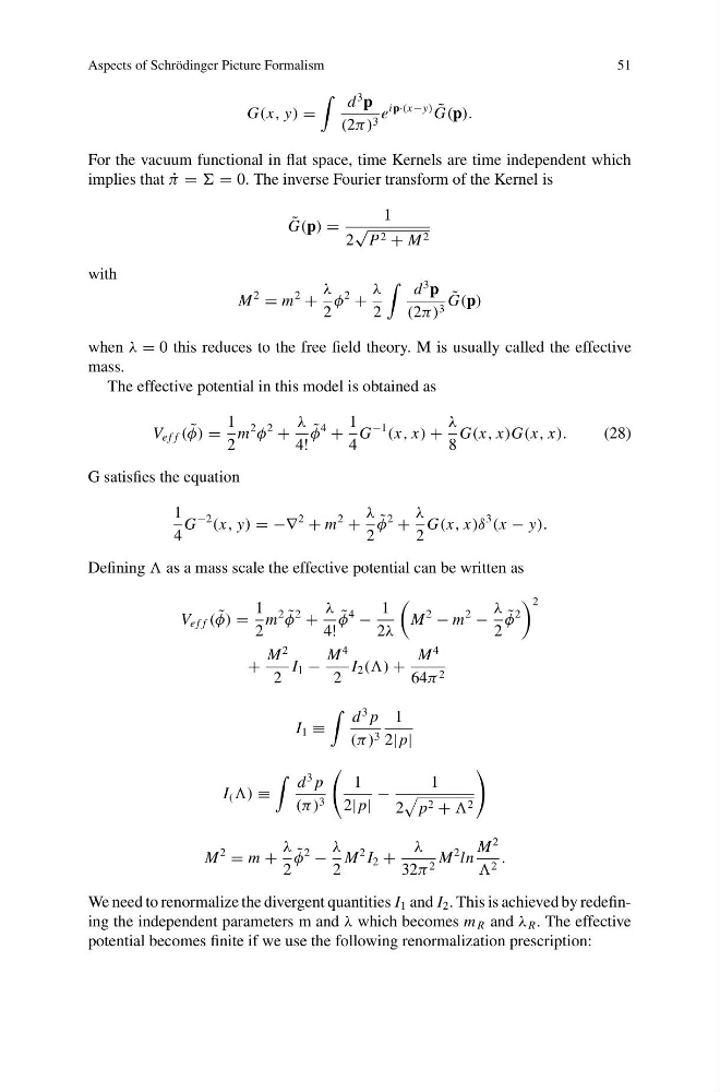
For the vacuum functional in flat space, time Kernels are time independent which
implies that ˙
π = = 0. The inverse Fourier transform of the Kernel is
˜
G(p) =
1
2
√
P 2 + M 2
with
M
2
= m
2
+
λ
2
φ
2
+
λ
2
d
3 p
(2π) 3
˜
G(p)
when λ = 0 this reduces to the free field theory. M is usually called the effective
mass.
The effective potential in this model is obtained as
V e f f ( ˜
φ) =
1
2
m
2
φ
2
+
λ
4!
˜
φ
4
+
1
4
G
−1
(x, x) +
λ
8
G(x, x)G(x, x).
(28)
G satisfies the equation
1
4
G
−2
(x, y) = −∇
2
+ m
2
+
λ
2
˜
φ
2
+
λ
2
G(x, x)δ
3
(x − y).
Defining as a mass scale the effective potential can be written as
V e f f ( ˜
φ) =
1
2
m
2 ˜
φ
2
+
λ
4!
˜
φ
4
−
1
2λ
M
2
− m
2
−
λ
2
˜
φ
2
2
+
M
2
2
I 1 −
M
4
2
I 2 (() +
M
4
64π 2
I 1 ≡
d
3 p
(π ) 3
1
2| p|
I ( ) ≡
d
3 p
(π ) 3
1
2| p|
−
1
2
p 2 + 2
M
2
= m +
λ
2
˜
φ
2
−
λ
2
M
2 I 2 +
λ
32π 2 M
2 ln
M
2
2 .
We need to renormalize the divergent quantities I 1 and I 2 . This is achieved by redefining the independent parameters m and λ which becomes m R and λ R . The effective
potential becomes finite if we use the following renormalization prescription:
51
G(x, y) =
d
3 p
(2π) 3 e
ip·(x−y) ˜
G(p).
For the vacuum functional in flat space, time Kernels are time independent which
implies that ˙
π = = 0. The inverse Fourier transform of the Kernel is
˜
G(p) =
1
2
√
P 2 + M 2
with
M
2
= m
2
+
λ
2
φ
2
+
λ
2
d
3 p
(2π) 3
˜
G(p)
when λ = 0 this reduces to the free field theory. M is usually called the effective
mass.
The effective potential in this model is obtained as
V e f f ( ˜
φ) =
1
2
m
2
φ
2
+
λ
4!
˜
φ
4
+
1
4
G
−1
(x, x) +
λ
8
G(x, x)G(x, x).
(28)
G satisfies the equation
1
4
G
−2
(x, y) = −∇
2
+ m
2
+
λ
2
˜
φ
2
+
λ
2
G(x, x)δ
3
(x − y).
Defining as a mass scale the effective potential can be written as
V e f f ( ˜
φ) =
1
2
m
2 ˜
φ
2
+
λ
4!
˜
φ
4
−
1
2λ
M
2
− m
2
−
λ
2
˜
φ
2
2
+
M
2
2
I 1 −
M
4
2
I 2 (() +
M
4
64π 2
I 1 ≡
d
3 p
(π ) 3
1
2| p|
I ( ) ≡
d
3 p
(π ) 3
1
2| p|
−
1
2
p 2 + 2
M
2
= m +
λ
2
˜
φ
2
−
λ
2
M
2 I 2 +
λ
32π 2 M
2 ln
M
2
2 .
We need to renormalize the divergent quantities I 1 and I 2 . This is achieved by redefining the independent parameters m and λ which becomes m R and λ R . The effective
potential becomes finite if we use the following renormalization prescription: