

Aspects of Schrödinger Picture Formalism
49
a(p)) 0 [φ] = 0.
First excited state
1 (φ) = Ca
†
(p 1 )) 0 (φ)
represents a state with one scalar particle of mass m and momentum p 1 and energy
ω p 1 . Even though the procedure given above analogous to conventional quantum
mechanics is exact for free fields the solution of Schrödinger equation in functional
form for interacting fields requires approximations. Most commonly used approximation is the variational approximation which we apply for the interacting fields.
5 Example of 4 Field
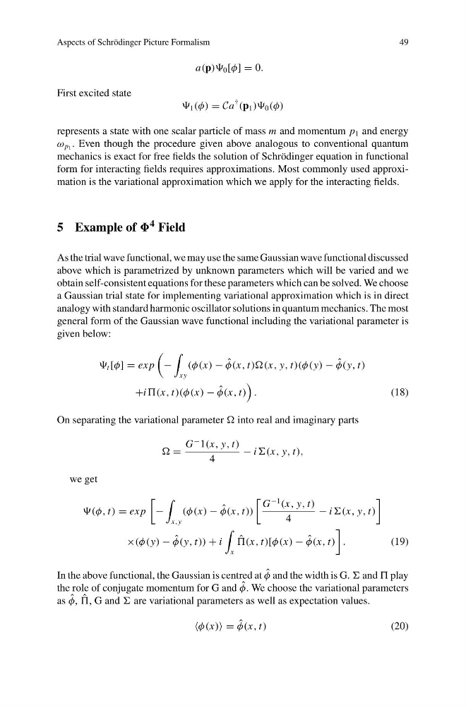
As the trial wave functional, we may use the same Gaussian wave functional discussed
above which is parametrized by unknown parameters which will be varied and we
obtain self-consistent equations for these parameters which can be solved. We choose
a Gaussian trial state for implementing variational approximation which is in direct
analogy with standard harmonic oscillator solutions in quantum mechanics. The most
general form of the Gaussian wave functional including the variational parameter is
given below:
t [φ] = ex p
−
xy
(φ(x) − ˆ
φ(x, t))(x, y, t)(φ(y) − ˆ
φ(y, t)
+i(x, t)(φ(x) − ˆ
φ(x, t)
.
(18)
On separating the variational parameter into real and imaginary parts
=
G
− 1(x, y, t)
4
− i(x, y, t),
we get
(φ, t) = ex p
−
x,y
(φ(x) − ˆ
φ(x, t))
G
−1
(x, y, t)
4
− i(x, y, t)
×(φ(y) − ˆ
φ(y, t)) + i
x
ˆ
(x, t)[φ(x) − ˆ
φ(x, t)
.
(19)
In the above functional, the Gaussian is centred at ˆ
φ and the width is G. and play
the role of conjugate momentum for G and ˆ
φ. We choose the variational parameters
as ˆ
φ, ˆ
, G and are variational parameters as well as expectation values.
φ(x) = ˆ
φ(x, t)
(20)
49
a(p)) 0 [φ] = 0.
First excited state
1 (φ) = Ca
†
(p 1 )) 0 (φ)
represents a state with one scalar particle of mass m and momentum p 1 and energy
ω p 1 . Even though the procedure given above analogous to conventional quantum
mechanics is exact for free fields the solution of Schrödinger equation in functional
form for interacting fields requires approximations. Most commonly used approximation is the variational approximation which we apply for the interacting fields.
5 Example of 4 Field
As the trial wave functional, we may use the same Gaussian wave functional discussed
above which is parametrized by unknown parameters which will be varied and we
obtain self-consistent equations for these parameters which can be solved. We choose
a Gaussian trial state for implementing variational approximation which is in direct
analogy with standard harmonic oscillator solutions in quantum mechanics. The most
general form of the Gaussian wave functional including the variational parameter is
given below:
t [φ] = ex p
−
xy
(φ(x) − ˆ
φ(x, t))(x, y, t)(φ(y) − ˆ
φ(y, t)
+i(x, t)(φ(x) − ˆ
φ(x, t)
.
(18)
On separating the variational parameter into real and imaginary parts
=
G
− 1(x, y, t)
4
− i(x, y, t),
we get
(φ, t) = ex p
−
x,y
(φ(x) − ˆ
φ(x, t))
G
−1
(x, y, t)
4
− i(x, y, t)
×(φ(y) − ˆ
φ(y, t)) + i
x
ˆ
(x, t)[φ(x) − ˆ
φ(x, t)
.
(19)
In the above functional, the Gaussian is centred at ˆ
φ and the width is G. and play
the role of conjugate momentum for G and ˆ
φ. We choose the variational parameters
as ˆ
φ, ˆ
, G and are variational parameters as well as expectation values.
φ(x) = ˆ
φ(x, t)
(20)