

48
K. P. Satheesh
G(x − y) =
1
2π 3
p
e
i p(x−y)
p 2 + m 2
(8)
E 0 =
1
2π 3
x
p
1
2
p 2 + m 2
(9)
0 [ ˆ
φ] = Cex p(
1
2 × 2π 3 )
p
ˆ
φ( p) ˆ
φ(− p)
p 2 + m 2
(10)
p 2 + m 2 ≡ ω p .
(11)
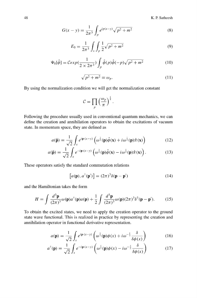
By using the normalization condition we will get the normalization constant
C =
p
ω p
π
1
4 .
Following the procedure usually used in conventional quantum mechanics, we can
define the creation and annihilation operators to obtain the excitations of vacuum
state. In momentum space, they are defined as
a( ˆ
p) =
1
√
2
x
e
ip·(x−y)
ω
1
2 (p) ˆ
φ(x) + iω
1
2 (p) ˆ
π(x)
(12)
a( ˆ
p) =
1
√
2
x
e
−ip·(x−y)
ω
1
2 (p) ˆ
φ(x) − iω
1
2 (p) ˆ
π(x)
.
(13)
These operators satisfy the standard commutation relations
a(p), a
†
(p
)
= (2π)
3
δ(p − p
)
(14)
and the Hamiltonian takes the form
H =
d
3 p
(2π) 3 ω(p)a
†
(p)a(p) +
1
2
d
3 p
(2π) 3 ω(p)(2π)
3
δ
3
(p − p
).
(15)
To obtain the excited states, we need to apply the creation operator to the ground
state wave functional. This is realized in practice by representing the creation and
annihilation operator in functional derivative representation.
a(p) =
1
√
2
x
e
ip·(x−y)
ω
1
2 (p)φ(x) + iω
−
1
2
δ
δφ(x)
(16)
a
†
(p) =
1
√
2
x
e
−ip·(x−y)
ω
1
2 (p)φ(x) − iω
−
1
2
δ
δφ(x)
(17)
K. P. Satheesh
G(x − y) =
1
2π 3
p
e
i p(x−y)
p 2 + m 2
(8)
E 0 =
1
2π 3
x
p
1
2
p 2 + m 2
(9)
0 [ ˆ
φ] = Cex p(
1
2 × 2π 3 )
p
ˆ
φ( p) ˆ
φ(− p)
p 2 + m 2
(10)
p 2 + m 2 ≡ ω p .
(11)
By using the normalization condition we will get the normalization constant
C =
p
ω p
π
1
4 .
Following the procedure usually used in conventional quantum mechanics, we can
define the creation and annihilation operators to obtain the excitations of vacuum
state. In momentum space, they are defined as
a( ˆ
p) =
1
√
2
x
e
ip·(x−y)
ω
1
2 (p) ˆ
φ(x) + iω
1
2 (p) ˆ
π(x)
(12)
a( ˆ
p) =
1
√
2
x
e
−ip·(x−y)
ω
1
2 (p) ˆ
φ(x) − iω
1
2 (p) ˆ
π(x)
.
(13)
These operators satisfy the standard commutation relations
a(p), a
†
(p
)
= (2π)
3
δ(p − p
)
(14)
and the Hamiltonian takes the form
H =
d
3 p
(2π) 3 ω(p)a
†
(p)a(p) +
1
2
d
3 p
(2π) 3 ω(p)(2π)
3
δ
3
(p − p
).
(15)
To obtain the excited states, we need to apply the creation operator to the ground
state wave functional. This is realized in practice by representing the creation and
annihilation operator in functional derivative representation.
a(p) =
1
√
2
x
e
ip·(x−y)
ω
1
2 (p)φ(x) + iω
−
1
2
δ
δφ(x)
(16)
a
†
(p) =
1
√
2
x
e
−ip·(x−y)
ω
1
2 (p)φ(x) − iω
−
1
2
δ
δφ(x)
(17)