

Aspects of Schrödinger Picture Formalism
47
i
∂∂(φ, t)
∂t
= H t) =
x
−
1
2
∂
2
∂φ 2 (x)
+
1
2
(∇φ)
2
+ V (φ)
(φ, t). (2)
For a time-dependent Hamiltonian, a separation of variables gives
t [φ] = e
−i Et
[φ]
and we are left with the functional eigenvalue problem
H
φ, −i
∂
∂φ
[φ] = E[φ].
4 Example of Non-interacting Scalar Field
We have V (φ) =
1
2
m
2
φ
2 and the free field Hamiltonian can be written as
H =
1
2
x
δ
2
δ(φ(x)δφ(x)
+ φ(x)(−∇
2
+ m
2
)φ(x)
.
(3)
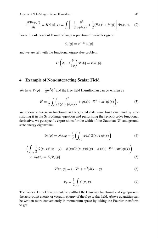
We choose a Gaussian functional as the ground state wave functional, and by substituting it in the Schrödinger equation and performing the second-order functional
derivative, we get specific expressions for the width of the Gaussian (G) and ground
state energy eigenvalue.
0 [φ] = N ex p −
1
2
x,y
φ(x)G(x, y)φ(y)
(4)
x,y
1
2
G(x, x)δ(x − y) − φ(x)G
2
(x, y)φ(y) + φ(x)(−∇
2
+ m
2
)φ(x)
× 0 (x) = E 0 0 [φ]
(5)
G
2
(x, y) = (−∇
2
+ m
2
)δ(x − y)
(6)
E 0 =
1
2
x
G(x, x).
(7)
The bi-local kernel G represent the width of the Gaussian functional and E 0 represent
the zero-point energy or vacuum energy of the free scalar field. Above quantities can
be written more conveniently in momentum space by taking the Fourier transform
to get
47
i
∂∂(φ, t)
∂t
= H t) =
x
−
1
2
∂
2
∂φ 2 (x)
+
1
2
(∇φ)
2
+ V (φ)
(φ, t). (2)
For a time-dependent Hamiltonian, a separation of variables gives
t [φ] = e
−i Et
[φ]
and we are left with the functional eigenvalue problem
H
φ, −i
∂
∂φ
[φ] = E[φ].
4 Example of Non-interacting Scalar Field
We have V (φ) =
1
2
m
2
φ
2 and the free field Hamiltonian can be written as
H =
1
2
x
δ
2
δ(φ(x)δφ(x)
+ φ(x)(−∇
2
+ m
2
)φ(x)
.
(3)
We choose a Gaussian functional as the ground state wave functional, and by substituting it in the Schrödinger equation and performing the second-order functional
derivative, we get specific expressions for the width of the Gaussian (G) and ground
state energy eigenvalue.
0 [φ] = N ex p −
1
2
x,y
φ(x)G(x, y)φ(y)
(4)
x,y
1
2
G(x, x)δ(x − y) − φ(x)G
2
(x, y)φ(y) + φ(x)(−∇
2
+ m
2
)φ(x)
× 0 (x) = E 0 0 [φ]
(5)
G
2
(x, y) = (−∇
2
+ m
2
)δ(x − y)
(6)
E 0 =
1
2
x
G(x, x).
(7)
The bi-local kernel G represent the width of the Gaussian functional and E 0 represent
the zero-point energy or vacuum energy of the free scalar field. Above quantities can
be written more conveniently in momentum space by taking the Fourier transform
to get