

4.3 Statistical Properties of Dynamic Speckle-Field Scattered …
335
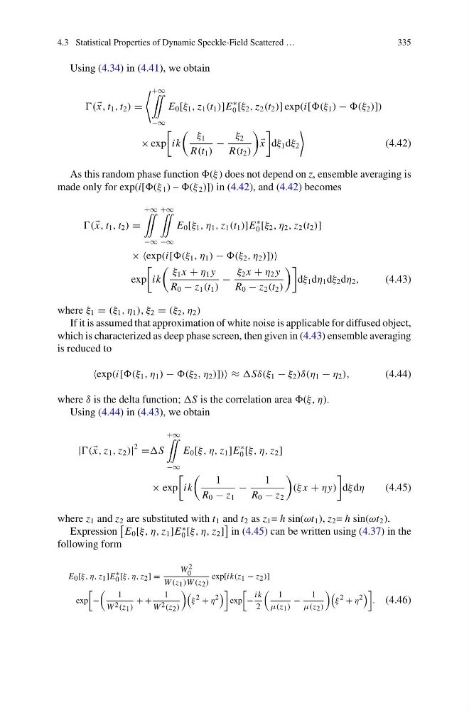
Using (4.34) in (4.41), we obtain
( x, t 1 , t 2 ) =
+∞
¨
−∞
E 0 [ξ 1 , z 1 (t 1 )]E
∗
0 [ξ 2 , z 2 (t 2 )] exp(i[(ξ 1 ) − (ξ 2 )])
× exp
ik
ξ 1
R(t 1 )
−
ξ 2
R(t 2 )
x
dξ 1 dξ 2
(4.42)
As this random phase function (ξ ) does not depend on z, ensemble averaging is
made only for exp(i[(ξ 1 ) – (ξ 2 )]) in (4.42), and (4.42) becomes
( x, t 1 , t 2 ) =
+∞
¨
−∞
+∞
¨
−∞
E 0 [ξ 1 , η 1 , z 1 (t 1 )]E
∗
0 [ξ 2 , η 2 , z 2 (t 2 )]
× ×exp(i[(ξ 1 , η 1 ) − (ξ 2 , η 2 )])
exp
ik
ξ 1 x + η 1 y
R 0 − z 1 (t 1 )
−
ξ 2 x + η 2 y
R 0 − z 2 (t 2 )
dξ 1 dη 1 dξ 2 dη 2 ,
(4.43)
where ξ 1 = (ξ 1 , η 1 ), ξ 2 = (ξ 2 , η 2 )
If it is assumed that approximation of white noise is applicable for diffused object,
which is characterized as deep phase screen, then given in (4.43) ensemble averaging
is reduced to
exp(i[(ξ 1 , η 1 ) − (ξ 2 , η 2 )]) ≈ Sδ(ξ 1 − ξ 2 )δ(η 1 − η 2 ),
(4.44)
where δ is the delta function; S is the correlation area (ξ, η).
Using (4.44) in (4.43), we obtain
|( x, z 1 , z 2 )|
2 =S
+∞
¨
−∞
E 0 [ξ, η, z 1 ]E
∗
0 [ξ, η, z 2 ]
× exp
ik
1
R 0 − z 1
−
1
R 0 − z 2
(ξ x + ηy)
dξ dη
(4.45)
where z 1 and z 2 are substituted with t 1 and t 2 as z 1 = h sin(ωt 1 ), z 2 = h sin(ωt 2 ).
Expression
E 0 [ξ, η, z 1 ]E
∗
0 [ξ, η, z 2 ]
in (4.45) can be written using (4.37) in the
following form
E 0 [ξ, η, z 1 ]E ∗
0 [ξ, η, z 2 ] =
W 2
0
W (z 1 )W (z 2 )
exp[ik(z 1 − z 2 )]
exp
−
1
W 2 (z 1 )
+ +
1
W 2 (z 2 )
ξ 2 + η 2
exp
−
ik
2
1
μ(z 1 )
−
1
μ(z 2 )
ξ 2 + η 2
. (4.46)
335
Using (4.34) in (4.41), we obtain
( x, t 1 , t 2 ) =
+∞
¨
−∞
E 0 [ξ 1 , z 1 (t 1 )]E
∗
0 [ξ 2 , z 2 (t 2 )] exp(i[(ξ 1 ) − (ξ 2 )])
× exp
ik
ξ 1
R(t 1 )
−
ξ 2
R(t 2 )
x
dξ 1 dξ 2
(4.42)
As this random phase function (ξ ) does not depend on z, ensemble averaging is
made only for exp(i[(ξ 1 ) – (ξ 2 )]) in (4.42), and (4.42) becomes
( x, t 1 , t 2 ) =
+∞
¨
−∞
+∞
¨
−∞
E 0 [ξ 1 , η 1 , z 1 (t 1 )]E
∗
0 [ξ 2 , η 2 , z 2 (t 2 )]
× ×exp(i[(ξ 1 , η 1 ) − (ξ 2 , η 2 )])
exp
ik
ξ 1 x + η 1 y
R 0 − z 1 (t 1 )
−
ξ 2 x + η 2 y
R 0 − z 2 (t 2 )
dξ 1 dη 1 dξ 2 dη 2 ,
(4.43)
where ξ 1 = (ξ 1 , η 1 ), ξ 2 = (ξ 2 , η 2 )
If it is assumed that approximation of white noise is applicable for diffused object,
which is characterized as deep phase screen, then given in (4.43) ensemble averaging
is reduced to
exp(i[(ξ 1 , η 1 ) − (ξ 2 , η 2 )]) ≈ Sδ(ξ 1 − ξ 2 )δ(η 1 − η 2 ),
(4.44)
where δ is the delta function; S is the correlation area (ξ, η).
Using (4.44) in (4.43), we obtain
|( x, z 1 , z 2 )|
2 =S
+∞
¨
−∞
E 0 [ξ, η, z 1 ]E
∗
0 [ξ, η, z 2 ]
× exp
ik
1
R 0 − z 1
−
1
R 0 − z 2
(ξ x + ηy)
dξ dη
(4.45)
where z 1 and z 2 are substituted with t 1 and t 2 as z 1 = h sin(ωt 1 ), z 2 = h sin(ωt 2 ).
Expression
E 0 [ξ, η, z 1 ]E
∗
0 [ξ, η, z 2 ]
in (4.45) can be written using (4.37) in the
following form
E 0 [ξ, η, z 1 ]E ∗
0 [ξ, η, z 2 ] =
W 2
0
W (z 1 )W (z 2 )
exp[ik(z 1 − z 2 )]
exp
−
1
W 2 (z 1 )
+ +
1
W 2 (z 2 )
ξ 2 + η 2
exp
−
ik
2
1
μ(z 1 )
−
1
μ(z 2 )
ξ 2 + η 2
. (4.46)