

3.4 Boundary Conditions of the Coupling Model
81
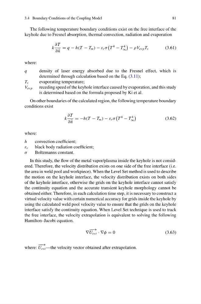
The following temperature boundary conditions exist on the free interface of the
keyhole due to Fresnel absorption, thermal convection, radiation and evaporation
k
∂ T
∂
n
= q − h(T − T m ) − ε r σ
T
4
− T
4
∞
− ρV ev p T v
(3.61)
where:
q
density of laser energy absorbed due to the Fresnel effect, which is
determined through calculation based on the Eq. (3.11);
T v
evaporating temperature;
V ev p
receding speed of the keyhole interface caused by evaporation, and this study
is determined based on the formula proposed by Ki et al.
On other boundaries of the calculated region, the following temperature boundary
conditions exist
k
∂ T
∂
n
= −h(T − T m ) − ε r σ
T
4
− T
4
∞
(3.62)
where:
h
convection coefficient;
ε r
black body radiation coefficient;
σ
Boltzmanns constant.
In this study, the flow of the metal vapor/plasma inside the keyhole is not considered. Therefore, the velocity distribution exists on one side of the free interface (i.e.
the area in weld pool and workpiece). When the Level Set method is used to describe
the motion on the keyhole interface, the velocity distribution exists on both sides
of the keyhole interface, otherwise the grids on the keyhole interface cannot satisfy
the continuity equation and the accurate transient keyhole morphology cannot be
obtained either. Therefore, in each calculation time step, it is necessary to construct a
virtual velocity value with certain numerical accuracy for grids inside the keyhole by
using the calculated weld pool velocity value to ensure that the grids on the keyhole
interface satisfy the continuity equation. When Level Set technique is used to track
the free interface, the velocity extrapolation is equivalent to solving the following
Hamilton–Jacobi equation.
∇
− − →
U ext · ∇φ = 0
(3.63)
where:
− − →
U ext —the velocity vector obtained after extrapolation.
81
The following temperature boundary conditions exist on the free interface of the
keyhole due to Fresnel absorption, thermal convection, radiation and evaporation
k
∂ T
∂
n
= q − h(T − T m ) − ε r σ
T
4
− T
4
∞
− ρV ev p T v
(3.61)
where:
q
density of laser energy absorbed due to the Fresnel effect, which is
determined through calculation based on the Eq. (3.11);
T v
evaporating temperature;
V ev p
receding speed of the keyhole interface caused by evaporation, and this study
is determined based on the formula proposed by Ki et al.
On other boundaries of the calculated region, the following temperature boundary
conditions exist
k
∂ T
∂
n
= −h(T − T m ) − ε r σ
T
4
− T
4
∞
(3.62)
where:
h
convection coefficient;
ε r
black body radiation coefficient;
σ
Boltzmanns constant.
In this study, the flow of the metal vapor/plasma inside the keyhole is not considered. Therefore, the velocity distribution exists on one side of the free interface (i.e.
the area in weld pool and workpiece). When the Level Set method is used to describe
the motion on the keyhole interface, the velocity distribution exists on both sides
of the keyhole interface, otherwise the grids on the keyhole interface cannot satisfy
the continuity equation and the accurate transient keyhole morphology cannot be
obtained either. Therefore, in each calculation time step, it is necessary to construct a
virtual velocity value with certain numerical accuracy for grids inside the keyhole by
using the calculated weld pool velocity value to ensure that the grids on the keyhole
interface satisfy the continuity equation. When Level Set technique is used to track
the free interface, the velocity extrapolation is equivalent to solving the following
Hamilton–Jacobi equation.
∇
− − →
U ext · ∇φ = 0
(3.63)
where:
− − →
U ext —the velocity vector obtained after extrapolation.