

78
3 Coupling Model and Numerical Computation Method of Keyhole and Weld Pool
n · ∇
− →
U · ·
n
= 0
(3.43)
Furtherly, based on Eq. (3.43), it can be deduced:
n ·
∇
− →
U
G
· ·
n = =
n ·
∇
− →
U
L
· ·
n
(3.44)
Finally, the discontinuity item
μ n · ∇
− →
U · ·
n
in Eqs. (3.44) and (3.35) can be
directly simplified into:
μ n · ∇
− →
U · ·
n
= [μ] n · ∇
− →
U · ·
n
(3.45)
Based on the principle that the tangential speed is continuous on the interface,
combining with Eq. (3.35), the following series of equations can be easily deduced:
μ t 1 · ∇
− →
U · ·
n
= [μ] t 1 · ∇
− →
U · ·
n
(3.46)
μ t 1 · ∇
− →
U ·
t 1
= [μ] t 1 · ∇
− →
U ·
t 1
(3.47)
μ t 1 · ∇
− →
U ·
t 2
= [μ] t 1 · ∇
− →
U ·
t 2
(3.48)
μ t 2 · ∇
− →
U · ·
n
= [μ] t 2 · ∇
− →
U · ·
n
(3.49)
μ t 2 · ∇
− →
U ·
t 1
= [μ] t 2 · ∇
− →
U ·
t 1
(3.50)
μ t 2 · ∇
− →
U ·
t 2
= [μ] t 2 · ∇
− →
U ·
t 2
(3.51)
μ n · ∇
− →
U ·
t 1
= −[μ] t 1 · ∇
− →
U · ·
n − ∇ s σ ·
t 1
(3.52)
μ n · ∇
− →
U ·
t 2
= −[μ] t 2 · ∇
− →
U · ·
n − ∇ s σ ·
t 2
(3.53)
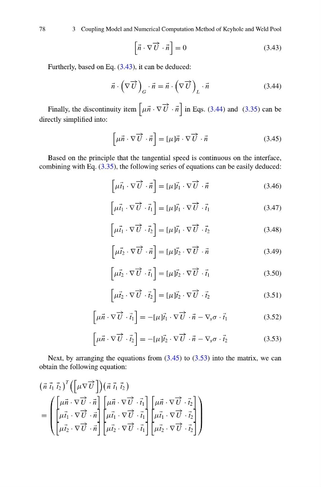
Next, by arranging the equations from (3.45) to (3.53) into the matrix, we can
obtain the following equation:
n
t 1
t 2
T
μ∇
− →
U
n
t 1
t 2
=
⎛
⎜
⎜
⎜
⎝
μ n · ∇
− →
U · ·
n
μ n · ∇
− →
U ·
t 1
μ n · ∇
− →
U ·
t 2
μ t 1 · ∇
− →
U · ·
n
μ t 1 · ∇
− →
U ·
t 1
μ t 1 · ∇
− →
U ·
t 2
μ t 2 · ∇
− →
U · ·
n
μ t 2 · ∇
− →
U ·
t 1
μ t 2 · ∇
− →
U ·
t 2
⎞
⎟
⎟
⎟
⎠
3 Coupling Model and Numerical Computation Method of Keyhole and Weld Pool
n · ∇
− →
U · ·
n
= 0
(3.43)
Furtherly, based on Eq. (3.43), it can be deduced:
n ·
∇
− →
U
G
· ·
n = =
n ·
∇
− →
U
L
· ·
n
(3.44)
Finally, the discontinuity item
μ n · ∇
− →
U · ·
n
in Eqs. (3.44) and (3.35) can be
directly simplified into:
μ n · ∇
− →
U · ·
n
= [μ] n · ∇
− →
U · ·
n
(3.45)
Based on the principle that the tangential speed is continuous on the interface,
combining with Eq. (3.35), the following series of equations can be easily deduced:
μ t 1 · ∇
− →
U · ·
n
= [μ] t 1 · ∇
− →
U · ·
n
(3.46)
μ t 1 · ∇
− →
U ·
t 1
= [μ] t 1 · ∇
− →
U ·
t 1
(3.47)
μ t 1 · ∇
− →
U ·
t 2
= [μ] t 1 · ∇
− →
U ·
t 2
(3.48)
μ t 2 · ∇
− →
U · ·
n
= [μ] t 2 · ∇
− →
U · ·
n
(3.49)
μ t 2 · ∇
− →
U ·
t 1
= [μ] t 2 · ∇
− →
U ·
t 1
(3.50)
μ t 2 · ∇
− →
U ·
t 2
= [μ] t 2 · ∇
− →
U ·
t 2
(3.51)
μ n · ∇
− →
U ·
t 1
= −[μ] t 1 · ∇
− →
U · ·
n − ∇ s σ ·
t 1
(3.52)
μ n · ∇
− →
U ·
t 2
= −[μ] t 2 · ∇
− →
U · ·
n − ∇ s σ ·
t 2
(3.53)
Next, by arranging the equations from (3.45) to (3.53) into the matrix, we can
obtain the following equation:
n
t 1
t 2
T
μ∇
− →
U
n
t 1
t 2
=
⎛
⎜
⎜
⎜
⎝
μ n · ∇
− →
U · ·
n
μ n · ∇
− →
U ·
t 1
μ n · ∇
− →
U ·
t 2
μ t 1 · ∇
− →
U · ·
n
μ t 1 · ∇
− →
U ·
t 1
μ t 1 · ∇
− →
U ·
t 2
μ t 2 · ∇
− →
U · ·
n
μ t 2 · ∇
− →
U ·
t 1
μ t 2 · ∇
− →
U ·
t 2
⎞
⎟
⎟
⎟
⎠