

3.5 Numerical Method
87
(a) Ray tracing process
(b) Cross-sectional distance field
(c) Energy distribution
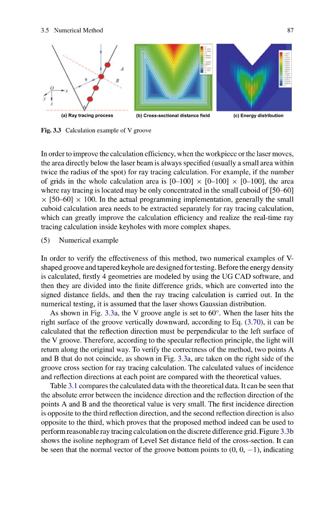
Fig. 3.3 Calculation example of V groove
In order to improve the calculation efficiency, when the workpiece or the laser moves,
the area directly below the laser beam is always specified (usually a small area within
twice the radius of the spot) for ray tracing calculation. For example, if the number
of grids in the whole calculation area is [0–100] × [0–100] × [0–100], the area
where ray tracing is located may be only concentrated in the small cuboid of [50–60]
× [50–60] × 100. In the actual programming implementation, generally the small
cuboid calculation area needs to be extracted separately for ray tracing calculation,
which can greatly improve the calculation efficiency and realize the real-time ray
tracing calculation inside keyholes with more complex shapes.
(5) Numerical example
In order to verify the effectiveness of this method, two numerical examples of Vshaped groove and tapered keyhole are designed for testing. Before the energy density
is calculated, firstly 4 geometries are modeled by using the UG CAD software, and
then they are divided into the finite difference grids, which are converted into the
signed distance fields, and then the ray tracing calculation is carried out. In the
numerical testing, it is assumed that the laser shows Gaussian distribution.
As shown in Fig. 3.3a, the V groove angle is set to 60°. When the laser hits the
right surface of the groove vertically downward, according to Eq. (3.70), it can be
calculated that the reflection direction must be perpendicular to the left surface of
the V groove. Therefore, according to the specular reflection principle, the light will
return along the original way. To verify the correctness of the method, two points A
and B that do not coincide, as shown in Fig. 3.3a, are taken on the right side of the
groove cross section for ray tracing calculation. The calculated values of incidence
and reflection directions at each point are compared with the theoretical values.
Table 3.1 compares the calculated data with the theoretical data. It can be seen that
the absolute error between the incidence direction and the reflection direction of the
points A and B and the theoretical value is very small. The first incidence direction
is opposite to the third reflection direction, and the second reflection direction is also
opposite to the third, which proves that the proposed method indeed can be used to
perform reasonable ray tracing calculation on the discrete difference grid. Figure 3.3b
shows the isoline nephogram of Level Set distance field of the cross-section. It can
be seen that the normal vector of the groove bottom points to (0, 0, −1), indicating
87
(a) Ray tracing process
(b) Cross-sectional distance field
(c) Energy distribution
Fig. 3.3 Calculation example of V groove
In order to improve the calculation efficiency, when the workpiece or the laser moves,
the area directly below the laser beam is always specified (usually a small area within
twice the radius of the spot) for ray tracing calculation. For example, if the number
of grids in the whole calculation area is [0–100] × [0–100] × [0–100], the area
where ray tracing is located may be only concentrated in the small cuboid of [50–60]
× [50–60] × 100. In the actual programming implementation, generally the small
cuboid calculation area needs to be extracted separately for ray tracing calculation,
which can greatly improve the calculation efficiency and realize the real-time ray
tracing calculation inside keyholes with more complex shapes.
(5) Numerical example
In order to verify the effectiveness of this method, two numerical examples of Vshaped groove and tapered keyhole are designed for testing. Before the energy density
is calculated, firstly 4 geometries are modeled by using the UG CAD software, and
then they are divided into the finite difference grids, which are converted into the
signed distance fields, and then the ray tracing calculation is carried out. In the
numerical testing, it is assumed that the laser shows Gaussian distribution.
As shown in Fig. 3.3a, the V groove angle is set to 60°. When the laser hits the
right surface of the groove vertically downward, according to Eq. (3.70), it can be
calculated that the reflection direction must be perpendicular to the left surface of
the V groove. Therefore, according to the specular reflection principle, the light will
return along the original way. To verify the correctness of the method, two points A
and B that do not coincide, as shown in Fig. 3.3a, are taken on the right side of the
groove cross section for ray tracing calculation. The calculated values of incidence
and reflection directions at each point are compared with the theoretical values.
Table 3.1 compares the calculated data with the theoretical data. It can be seen that
the absolute error between the incidence direction and the reflection direction of the
points A and B and the theoretical value is very small. The first incidence direction
is opposite to the third reflection direction, and the second reflection direction is also
opposite to the third, which proves that the proposed method indeed can be used to
perform reasonable ray tracing calculation on the discrete difference grid. Figure 3.3b
shows the isoline nephogram of Level Set distance field of the cross-section. It can
be seen that the normal vector of the groove bottom points to (0, 0, −1), indicating