

3.10 Computing a Green’s Function for a Layered Workpiece
83
with
R 1 = (v 20 , v 40 )
R 2 = (v 10 , v 30 )
S (i) =
v
(i)
1 , v
(i)
3 , v
(i)
2 , v
(i)
4
E (i) =
⎡
⎢
⎢
⎣
e λ 1 h i 0
0
0
0 e λ 3 h i 0
0
0
0 e −λ 1 h i 0
0
0
0 e −λ 3 h i
⎤
⎥
⎥
⎦
h i = z i − z i−1
X =
˜
d, ˜
f , c (1) , e (1) , d (1) , f (1) , · · · , c (10) , e (10) , d (10) , f (10) , g, h
T
˜
d = de λ 0 z
˜
f = f e λ 0 z
Y =
−v 10 c − v 30 e
0 40×1
e −λ 0 z
.
(3.24)
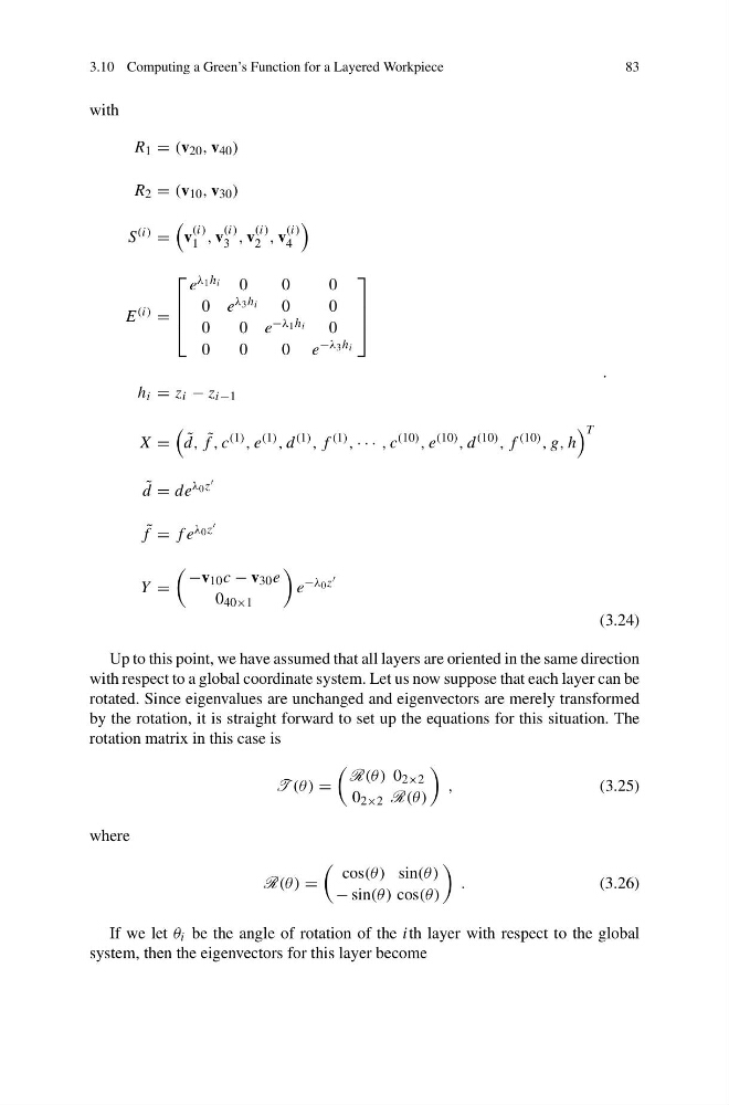
Up to this point, we have assumed that all layers are oriented in the same direction
with respect to a global coordinate system. Let us now suppose that each layer can be
rotated. Since eigenvalues are unchanged and eigenvectors are merely transformed
by the rotation, it is straight forward to set up the equations for this situation. The
rotation matrix in this case is
T (θ ) =
R(θ ) 0 2×2
0 2×2 R(θ )
,
(3.25)
where
R(θ ) =
cos(θ ) sin(θ )
− sin(θ ) cos(θ )
.
(3.26)
If we let θ i be the angle of rotation of the ith layer with respect to the global
system, then the eigenvectors for this layer become
83
with
R 1 = (v 20 , v 40 )
R 2 = (v 10 , v 30 )
S (i) =
v
(i)
1 , v
(i)
3 , v
(i)
2 , v
(i)
4
E (i) =
⎡
⎢
⎢
⎣
e λ 1 h i 0
0
0
0 e λ 3 h i 0
0
0
0 e −λ 1 h i 0
0
0
0 e −λ 3 h i
⎤
⎥
⎥
⎦
h i = z i − z i−1
X =
˜
d, ˜
f , c (1) , e (1) , d (1) , f (1) , · · · , c (10) , e (10) , d (10) , f (10) , g, h
T
˜
d = de λ 0 z
˜
f = f e λ 0 z
Y =
−v 10 c − v 30 e
0 40×1
e −λ 0 z
.
(3.24)
Up to this point, we have assumed that all layers are oriented in the same direction
with respect to a global coordinate system. Let us now suppose that each layer can be
rotated. Since eigenvalues are unchanged and eigenvectors are merely transformed
by the rotation, it is straight forward to set up the equations for this situation. The
rotation matrix in this case is
T (θ ) =
R(θ ) 0 2×2
0 2×2 R(θ )
,
(3.25)
where
R(θ ) =
cos(θ ) sin(θ )
− sin(θ ) cos(θ )
.
(3.26)
If we let θ i be the angle of rotation of the ith layer with respect to the global
system, then the eigenvectors for this layer become